Chapter 4 Confidence Intervals and Bootstrap
The following packages are required for this chapter.
This chapter first provides an overview of the terms and concepts surrounding Confidence Intervals. It then provides an overview of the most commonly used theory-based confidence interval techniques, providing some mathematical perspective but not a rigorous mathematical treatment of the subject. Following that, simulation-based confidence interval techniques are introduced featuring the Bootstrap method. After providing contrast between the theory-based and simulation-based techniques, the Infer package is introduced as a tool for constructing simulation-based confidence intervals.
4.1 Terms and Concepts
Recall that a main goal of inferential statistics is to infer about an unknown population parameter (mean or proportion, for example) by taking a random sample from the population. The corresponding statistic computed from the sample is called a point estimate for the unknown population parameter. An important question: How much confidence is there that the unknown population parameter is actually close to the point estimate? If you are “lucky” and the random sample very closely represents the population, then the unknown population parameter should be relatively close to the point estimate. But on the other hand, the point estimate might not be very close. Random sampling involves inherent sampling variation (the luck of the draw in card game), hence the need for some notion of confidence regarding a point estimate.
As discussed at length in the previous Chapter, a Sampling Distribution quantifies the sampling variation by providing a probability model for all samples of size \(n\) taken from the population. The CLT guarantees that the sampling distribution can be assumed to be normal if the sample size \(n\) is sufficiently large. The standard deviation of a sampling distribution is called the Standard Error (SE). The SE gives the “spread” of the sampling distribution, effectively quantifying sampling error. It follows logically that the SE will be key in addressing the issue of confidence as it pertains to point estimates. The table below summarizes some relevant information and notation from the previous Chapter.
| Statistic | Point Estimate From Sample | Population Parameter(s) | Standard Error from CLT |
|---|---|---|---|
| Mean | \(\bar{x}\) (or \(\hat{\mu}\)) | \(\mu\), \(\sigma\) | \(SE = \frac{\sigma}{\sqrt{n}}\) |
| Proportion | \(\hat{p}\) | \(p\) | \(SE = \sqrt{\frac{p(1-p)}{n}}\) |
The next logical step is to create a Confidence Interval (CI) surrounding the point estimate that “probably” contains the unknown population parameter based upon a certain confidence level, often 95% or 99%. For the sake of discussion, let’s consider a 95% confidence level for an a population mean. The 68-95-99.7 principle for normal distributions indicates that the center 95% of the sampling distribution is within about 2 standard deviations of \(\mu\), the mean of sampling distribution. Thus, if you take a size \(n\) sample from the population, you can be 95% confident that its mean \(\bar{x}\) falls within about \(\pm 2 SE\) of \(\mu\).
But you typically don’t know \(\mu\), which is why a sample is taken to infer about it. So instead, translate the \(\pm 2 SE\) to be centered around the known point estimate \(\bar{x}\). The result is a 95% CI of the form \([\bar{x}-2\cdot SE\;,\; \bar{x}+2\cdot SE]\), which is an interval of real numbers centered around the point estimate \(\bar{x}\). There is then 95% confidence that the CI constructed from the observed sample actually contains the unknown population mean \(\mu\).
The 68-95-99.7 principle for normal distributions is only meant to be a quick rule of thumb, so it contains some rounding error. Thus, the \(\pm 2\) mentioned above isn’t quite accurate enough for the purpose of confidence intervals. It’s easy to apply R’s built-in qnorm (quantile norm) function (discussed in Section 2.6) to a standard normal \(N(0,1^2)\) distribution to produce the precise value. Outside of the middle .95 area, the left and right tails have a combined area of .05, leaving an area of .025 in each tail. The computation below shows that 95% of the area of any normal curve is within 1.96 sd’s of the mean.
For a concrete example, we return to the data on dragon wingspans that was featured in Section 3.3. Here’s a quick summary:
- The population was known with mean \(\mu=7.34\) and standard deviation \(\sigma=2.23\)
- A random \(n=75\) sample was taken and the sample mean (point estimate) was \(\bar{x}=6.96\).
- The sampling distribution was calculated using the CLT to be \(N(7.34,(.257)^2)\), where \(SE=\frac{\sigma}{\sqrt{n}}=\frac{2.23}{\sqrt{75}}=.257\).
Thus, a 95% confidence interval centered on \(\bar{x}\) is calculated as follows:
\([\bar{x} - 1.96\cdot SE \; , \; \bar{x} + 1.96\cdot SE] = [6.96 - 1.96\cdot .257 \; , \; 6.96 + 1.96\cdot .257] = [6.46\; , \;7.46]\)
Assuming we didn’t already know the population mean, we could say with 95% confidence that it is contained in the interval \([6.46,7.46]\).
Of course, the main benefit of sampling from a known population for this example is being able to see how well-founded that confidence actually is. For this sample, the confidence lives up to the hype since the population mean of \(\mu=7.34\) is easily inside the CI. That’s not really surprising since the sampling distribution z-score for \(\bar{x}\) was calculated in Section 3.3 to be \(z=(6.96-7.34)/.257=-1.5\), which means \(\bar{x}\) is only about 1.5 SE’s away from the expectation \(\mu=7.34\). From that we concluded that the particular sample was a reasonable representative of the population. Both that observation and the CI constructed above, show that the sample was reasonably representative of the population.
The CI calculation above used an SE multiplier of 1.96 which is specific to a 95% CI. For another example, consider a 99% SE multiplier which can be similarly calculated from a Standard Normal N(01) distribution as shown below.
Figure 4.1 shows the multipliers for the most common confidence levels used in practice.
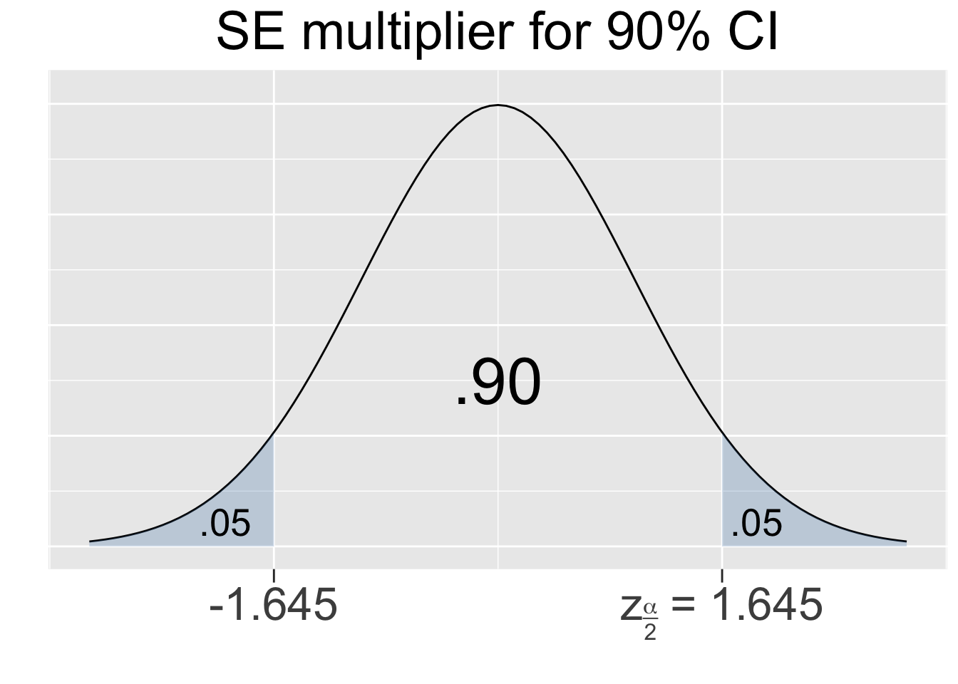
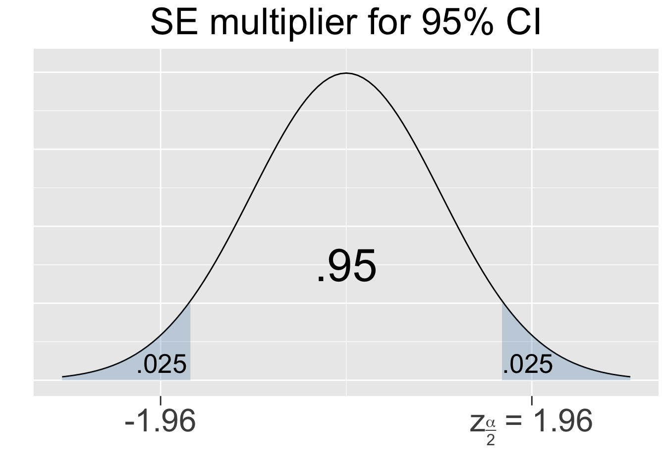

Figure 4.1: SE Multipliers for common Confidence Levels
The SE multipliers in Figure 4.1 are labeled \(z_{\alpha/2}\) in keeping with standard notation. The variable \(z\) is used since the multipliers are calculated using the Standard Normal N(01) distribution, also called the Z-distribution. For a given confidence level, say 95%, the quantity alpha is defined as \(\alpha = 1-.95=.05\) which is the shaded area under both tails combined. Thus, the area under each separate tail is then \(\alpha/2=.025\).
In general, a confidence interval is expressed as follows, where the SE multiplier \(z_{\alpha/2}\) is determined by the confidence level.
\[\left[\bar{x}-z_{\alpha/2}\cdot SE\; , \; \bar{x}+z_{\alpha/2}\cdot SE\right]\]
The quantity \(z_{\alpha/2}\cdot SE\) is sometimes called the sampling Margin of Error (MoE). The center of the CI is the point estimate \(\bar{x}\), and the endpoints of the CI are \(\bar{x} \pm MoE\). Thus, reporting a CI as an interval of numbers is equivalent to reporting the point estimate and the sampling MoE. In fact, that’s how CIs are usually reported for percentages (proportions) in public opinion polling.
We’ll again go back to the usual state of affairs when doing inference and assume that the population mean for dragon wingspans is unknown. The stated conclusion about the \([6.46,7.46]\) dragon wingspan CI computed above was that there is “95% confidence” that the CI contains the population mean. As you saw, computing the CI was not difficult. Surprisingly, it is a more difficult task to answer the following question: What does “95% confidence” actually mean in this context? Clarifying the notion of confidence as it pertains to Cls is important because misconceptions are quite common.
We’ll answer the question of what “confidence” means for a 95% CI, but the answer generalizes to any confidence level. If you take one sample of \(n=75\) dragons from the population, the expectation for the sample mean \(\bar{x}\) is the population mean \(\mu\). That’s just the best guess. The actual value of \(\bar{x}\) is likely different from \(\mu\), and there is no way of knowing how different when \(\mu\) is unknown.
So we turn to the sampling distribution - the probability model for the space of all possible samples of size \(n=75\) from the dragon population. The middle 95% of the sampling distribution defines an x-axis interval that should contain most dragon sample \(\bar{x}\) values, all but about 5% of them. That interval is approximately \(\mu\pm z_{\alpha/2}\cdot SE\). Since \(\mu\) is unknown, we don’t know exactly where this middle 95% interval is, but \(MoE = z_{\alpha/2}\cdot SE\) does provide an estimate for how wide it is - roughly 2 MoE centered around the unknown \(\mu\).
Since the 95% CI is \(\bar{x}\pm z_{\alpha/2}\cdot SE\), we see that the CI is the middle 95% interval from the sampling distribution, just re-centered on the specific sample mean \(\bar{x}\), a known quantity. That concept is summarized in the following table.
| Middle 95% of Sampling Distribution | \(\mu\) Unknown | 95% Confidence Interval |
|---|---|---|
| \(\left[\mu-z_{\alpha/2}\cdot SE\; , \; \mu+z_{\alpha/2}\cdot SE\right]\) | \(\implies\) | \(\left[\bar{x}-z_{\alpha/2}\cdot SE\; , \; \bar{x}+z_{\alpha/2}\cdot SE\right]\) |
Since about 95% of all possible sample means are expected to fall in the \(\mu\)-centered 95% of the sampling distribution, it follows that the unknown \(\mu\) is expected to be contained in about 95% of all possible \(\bar{x}\) centered CIs.
There’s an old expression, most versions of which say something like someone “can’t see the forest for the trees.” That is, looking too much at the fine details can cause someone to miss the overall big picture of the forest as a whole. The same is true about focusing on the CI formula details at the expense the more general picture. The above discussion is summarized below, just without some of the trees.
CI Perspective
The standard deviation (SE) of the sampling distribution quantifies the sampling error. The sampling MoE - a multiple of the SE - defines the center, say 95%, of the sampling distribution. In the space of all possible samples, most (all but 5%) sample means are expected to fall into that middle 95% centered around \(\mu\). But \(\mu\) is unknown, so that central 95% interval is instead recentered around \(\bar{x}\) resulting in a 95% CI. The result is that 95% of random samples are expected to result in a CI that contains \(\mu\), with the other 5% of them being the “unlucky” ones with the largest sampling error.
So the notion of “confidence” in this context boils down to what is expected in the space of all possible CIs - that about 95% of them should contain the unknown \(\mu\). A good way to visualize this expectation is to run a simulation of 100 random samples and and observe the resulting CIs. Figure 4.2 shows the result of such a simulation resulting from 100 different size \(n=75\) samples taken randomly from the dragon population. Each horizontal line shows the extent of one CI, with the dot in the center being the mean \(\bar{x}\) of the sample. The dotted vertical line is the dragon population wingspan mean \(\mu\), which we have conveniently remembered again for the sake of this simulation. A “hit” means the CI (colored grey) actually contains \(\mu\), whereas a “miss” means the CI (colored red) doesn’t. The misses are effectively “unlucky” samples that don’t represent the population very well.
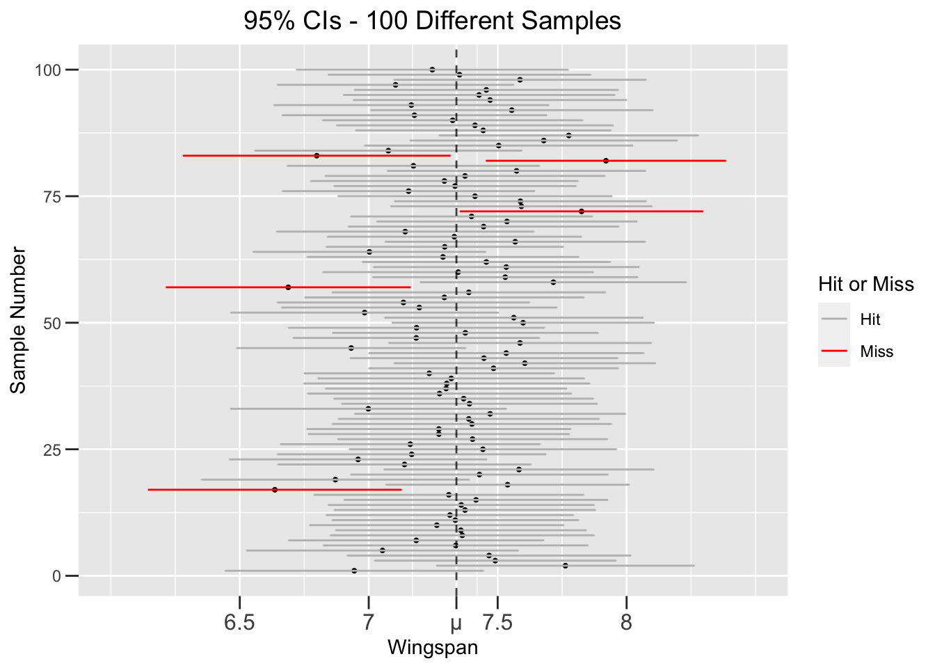
Figure 4.2: Simulation of 100 different 95% Confidence Intervals
The simulation in Figure 4.2 resulted in exactly 5 misses, which matches the expectation that 100 different 95% CIs should contain 95 hits. But that’s just what’s expected, not a guarantee. If the sample simulation is run again, there might be 4 misses, 6 misses, or some other number. That’s sampling variation at work. It’s too messy to plot a similar 1,000 CI simulation, but the expectation would be 950 hits and 50 misses. Again, the simulation might not result in the exact expected number of misses, but the law of large numbers says there would be a better chance of matching the expectation with a larger simulation
Meaning of 95% Confidence
If many samples of size \(n\) are taken from the population and a 95% CI calculated from each, it is expected that about 95% of them will contain the unknown population parameter.
Notice that the meaning of “confidence” doesn’t even apply to a single CI. Key point: if the population mean is truly an unknown quantity, then there is literally no way to assign a probability to whether or not a specific CI contains it. Period. Thus, the notion of 95% Confidence does not indicate a specific probability about a specific CI. Rather, it’s an expectation about the space of all possible 95% CIs (constructed from samples of the same size of course).
Keeping that in mind, 95% Confidence
- does NOT indicate the probability that a CI contains the unknown population parameter is .95.
- does NOT indicate that 95% of samples will result in a CI that contains the unknown population parameter.
Remove the “NOT” from each statement above, and the resulting statements would be false, resulting in the most common misconceptions about Cls. Without the NOT, the first one is just totally wrong, being impossible to calculate. Without the NOT, the second one is closer to being true, and actually true if rephrased in terms of expectation instead of a guarantee. That’s a very subtle point, which emphasizes why it’s hard to define what confidence means in this context.
The answer provided above to the main question of what “confidence” means for CIs is not very satisfying in the sense that it doesn’t say anything specific about a particular CI. Rather, it’s about what 95% confidence means with respect to expectations from a probability model (sampling distribution) for the space of all possible size \(n\) samples from the population. If we forget about all the trees and view the forest from 30,000 feet above, then 95% confidence means that we hope the CI doesn’t come from the 5% of the most unlucky-non-population-representing samples.
The final observations about confidence intervals presented in this section are much more readily explained. Figure 4.3 depicts the effect of sample size on confidence intervals. It shows 95% CIs constructed from 4 different random samples of increasing sizes taken from the dragon population. Notice that the width of the Cls decrease as the sample size increases.
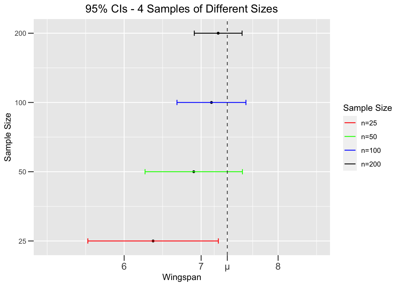
Figure 4.3: Effect of Sample Size on Confidence Intervals
The effect of sample size is readily apparent from the standard error formula \(SE = \frac{\sigma}{\sqrt{n}}\). A larger \(n\) makes the bottom of the fraction larger, which makes the entire fraction (the SE) smaller. Thus for a given confidence level, say 95%, a smaller SE makes a smaller CI. A smaller CI (from larger sample) is better since it gives a more precise interval estimate for the unknown population parameter. That’s not surprising since a larger sample tends to more accurately represent the population than a small one.
But wait a minute! For a given confidence level, wouldn’t a larger CI - a wider interval of numbers - from a small sample be more likely to contain the unknown \(\mu\)? Not really, because the mean \(\bar{x}\) from a small sample is less likely to be close to \(\mu\), which in turn makes the CI less likely to contain \(\mu\). Figure 4.3 shows exactly that. The small-sample CI (red on the bottom) is wider, but still misses \(\mu\) because its point estimate \(\bar{x}\) is way off target. The big-sample CI (black at top) is the smallest, but still hits \(\mu\) since \(\bar{x}\) is closer. In inferential statistics, larger samples are always desirable as they give more precise estimates about the population.
Figure 4.4 shows the effect of confidence level on CI width. It shows 4 CIs, each with a different confidence level, but all constructed from the SAME sample. Since each CI is from the same sample, the SE is the same in each CI calculation. But a larger confidence level gives a larger \(z_{\alpha/2}\), hence a wider CI. A wider CI provides a less precise interval estimate for \(\mu\). But in this case the loss of precision could be offset by a higher confidence in the CI. It’s a trade-off: more confidence but less accuracy, or less confidence and more accuracy.
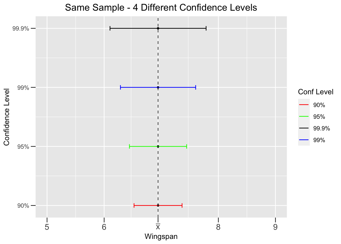
Figure 4.4: Effect of Confidence Level on Confidence Intervals
That trade-off is simply stated, but the finer points about its implications are somewhat complicated. We’ll defer discussion of that until the chapter on hypothesis tests. But we can quickly address the ramifications of too much confidence. With human personality traits, having lots of confidence is generally good. But too much confidence can lead one to make unwise decisions, or even reckless ones. He’s so confident in his chainsaw juggling skills, that … Let’s hope that confidence is well founded.
Similarly, in statistics a high confidence level such as 95% is also generally good. But how about 99.99%, 99.999%, or even 100% confidence? As Figure 4.4 demonstrates, 99.99% or 99.999% would produce Cls so wide as to not provide a very precise interval estimate for \(\mu\). A 100% confidence level actually results in a CI of \((-\infty,\infty)\) which covers the whole real number line. It’s not useful at all to be 100% confident that an unknown population mean \(\mu\) is somewhere between positive and negative infinity.
The last point we’ll make about the “choice” of confidence level, is that it’s often not really a choice. The confidence level - usually between 90%-99% - is often dictated by the research standards for a certain type of analysis, or even the nature of the research field itself. Social science research may have different confidence level standards than medical research, where wrong conclusions drawn from a sample can have deadly consequences. In most cases, the confidence level is simply determined by what is customary in the given situation. When in doubt, 95% is usually the best choice.
4.2 Single Proportions
As demonstrated in the previous section, a confidence interval is constructed using multiples of the SE of the sampling distribution. The SE formulas are computed from population parameters. However, the main reason statistical inference is practiced is that you don’t know the population parameters.
That’s why you take a random sample! That highlights an obvious, significant issue: You can’t use an unknown population parameter to compute the SE for a CI if you don’t know the population parameter. The best solution to that problem is to simply substitute the observed \(\hat{p}\) for \(p\) and calculate the approximate SE.
\[SE \approx \sqrt{\frac{\hat{p}(1-\hat{p})}{n}}\]
It can be proven mathematically that as \(n\) gets large (\(n\rightarrow\infty\)), the difference between computing the SE with \(\hat{p}\) and computing it \(p\) asymptotically approaches 0. That is, the error induced by the \(\hat{p}\) substitution for the SE decreases toward 0 as \(n\) increases.
Recall from Section 3.5 that the CLT for proportions already depends upon approximating a binomial distribution with a normal one. This substitution then adds another approximation on top of that. Since the conditions for a reasonable normal approximation to a binomial (\(np\gt 10\) and \(n(1-p) \gt 10\)) already assure n to be relatively large, the same conditions are usually considered sufficient to construct confidence intervals for proportions by substituting \(\hat{p}\) for \(p\) into the SE formula.
Assuming that \(p\) is unknown, the mathematics behind Cls for proportions require the following assumptions to hold.
ASSUMPTIONS for Proportion CI:
- The sample size \(n\) is sufficiently large, and \(\hat{p}\) is not close to 0 or 1. Satisfying the \(np\gt 10\) and \(n(1-p) \gt 10\) criteria is usually sufficient unless \(\hat{p}\) is close to 0 or 1, in which case even larger \(n\) is desirable.
- When sampling without replacement, in survey/polling for example, the sample size must be negligible compared to the population size to ensure the Bernoulli trials are approximately independent.
Under these assumptions, the CI for an unknown population proportion \(p\) is shown below.
\[ p\in \left[\; \hat{p} - z_{\alpha/2}\sqrt{\frac{\hat{p}(1-\hat{p})}{n}} \;\;\;\; , \;\; \;\; \hat{p} + z_{\alpha/2}\sqrt{\frac{\hat{p}(1-\hat{p})}{n}}\;\;\right]\]
Above, \(z_{\alpha/2}\) is the appropriate SE multiplier from the standard normal N(0,1) distribution. In short, the above CI is \(\left[\hat{p}-z_{\alpha/2}\cdot SE\; , \; \hat{p}+z_{\alpha/2}\cdot SE\right]\).
The following example uses real data from the General Social Survey (GSS), a survey conducted every two years (in even years) coordinated by the University of Chicago with contributing researchers from around the USA. They make the data publicly available for free. See https://gss.norc.org if you are curious. It’s a vast data source that provides 10’s of thousands of records (surveys) and thousands of columns (variables) going back decades.
The CSV file loaded below contains a subset of the data that contains over 4000 records and 6 columns. This population from which the sample was drawn are people in the USA.
gss_survey <- read_csv("http://www.cknuckles.com/statsprogramming/data/gss_survey_data.csv")
gss_survey
## # A tibble: 4,146 × 6
##     year tvhours party            income         status        workhours
##    <dbl>   <dbl> <chr>            <chr>          <chr>             <dbl>
##  1  2010       1 Not str democrat $25000 or more Never married        55
##  2  2010       0 Not str democrat $7000 to 7999  Never married        45
##  3  2010       1 No answer        Refused        Never married        48
##  4  2010       4 Strong democrat  $20000 - 24999 Never married        26
##  5  2010      NA Strong democrat  $25000 or more Married              40
##  6  2010       0 Ind,near dem     $25000 or more Never married        50
##  7  2010       0 Independent      $25000 or more Divorced             40
##  8  2010       5 Ind,near dem     $25000 or more Married              NA
##  9  2010       0 Not str democrat $25000 or more Married              20
## 10  2010       1 Not str democrat $1000 to 2999  Never married        25
## # ℹ 4,136 more rows
For an example on proportions, we’ll use only the tvhours column and only the survey results from 2018, the most recent year of GSS data available at the time this was written. so some data wrangling is in order. The code below creates a much smaller table named tvhours_2018 with only the survey records from 2018 and thetvhours variable, which records how many hours per week the survey participants watch on average. Notice that the last line removes all NA values in the tvhours column. Perhaps some people without a TV didn’t answer the question instead of just reporting 0.
It’s always a good idea to visualize data before analyzing it. The summary below of the resulting 833 records shows that some people don’t watch any TV, while at least one person reported watching TV almost all day for 20 hours on average. The right skew (hump on left) in the data is obvious from the histogram. The summary confirms the right skew since the mean of the data is to the right of the median.
ggplot(data = tvhours_2018, mapping = aes(x = tvhours)) +
  geom_histogram( bins=15, color = "white")

summary(tvhours_2018$tvhours)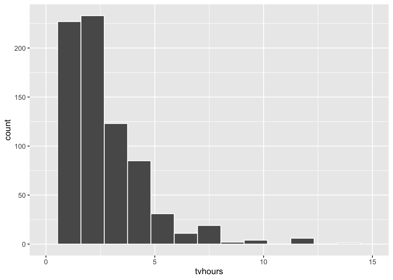
##    Min. 1st Qu.  Median    Mean 3rd Qu.    Max.
##    0.00    1.00    2.00    2.32    3.00   20.00
For the purposes of this example, we’ll define a “couch potato” as anyone that reported TV viewing greater than or equal to the 75th percentile - 3 hours per day. The objective is to create a 99% CI, centered around the observed proportion \(\hat{p}\) of couch potatoes in this sample of \(n=833\) people. First, the data needs to be described using the terminology of success/failure Bernoulli trials and proportions. Each record (one person surveyed) is just a tvhours number. But a comparison like \(tvhours >= 3\) is either true or false, or better yet success or failure. So in Bernoulli terminology, being a couch potato is actually a success! (Most parents might not see it that way.) By applying that comparison to each tvhours number, each record effectively becomes a success/failure Bernoulli trial.
The \(\hat{p}\) from the survey data is easily computed as shown below using \(tvhours >= 3\) as the Bernoulli success criteria.
tvhours_2018 %>%
  summarize(
    num_couch_potatoes = sum(tvhours >= 3),
    n = n(),
    p_hat = num_couch_potatoes/n   # proportion of couch potatoes
  )
## # A tibble: 1 × 3
##   num_couch_potatoes     n p_hat
##                <int> <int> <dbl>
## 1                283   833 0.340
The final proportion p_hat of couch potatoes in the above code is simply the number of them divided by the sample size \(n\). The number of couch potatoes is calculated by sum(tvhours >= 3) which adds a 1 to num_couch_potatoes if tvhours >= 3 is true, otherwise a 0 is added. A call to the sum() function like sum(tvhours) would simply add up all the hours, but placing a Boolean (T/F) expression inside the sum results in adding 1’s and 0’s corresponding to the truth values.
The sample size \(n=833\) is easily large enough to meet the required assumptions since \(n\hat{p} = 833\times.340 = 283 > 10\) and \(n(1-\hat{p})\) is even larger. Thus, a 99% CI can be calculated by substituting \(\hat{p}=.340\) into the SE formula as follows.
In the above CI calculation, the SE multiplier of 2.58 is the \(z_{\alpha/2}\) value for a 99% CI as shown in Figure 4.1 and the lower/upper endpoints of the resulting CI of [.298,.382] are combined into a vector to print them on one line in the output. The conclusion is that there is a 99% probability that the unknown proportion \(p\) of couch potatoes in the USA would be between 29.8% and 38.2%. To be fair, many of these so called “couch potatoes” could be educationally motivated high-volume watchers of non-fiction documentaries.
You may have noticed that the proportions near the end of the previous paragraph are given as percentages, which is technically an abuse of terminology. However, proportion and percentage are just two different ways of expressing the same quantity. In political polling, and other types of public opinion polling, it’s common to report proportions in percentage form as it’s more intuitive for the average person.
Suppose for example that a political poll of \(n=1000\) people yields a sample proportion of \(\hat{p}=.55\) that support the Republican candidate. That would typically be reported in the news as 55% of 1000 likely voters polled support the candidate. Somewhere in smaller print it would then say the poll has a margin of error of approximately \(\pm 3\). The most common confidence level used in polling is 95%, so the \(\pm 3%\) simply refers to the width of the 95% CI. Using the margin of error of approximately \(\pm 3%\) (computed below as approximately .03), the CI is then roughly [52%,58%] in keeping with percentages.
SE <- sqrt((.55*(1-.55))/1000)

poll_margin_of_error <- (1.96*SE)  # Half of width of the 95% CI
poll_margin_of_error
## [1] 0.0308
Recall the discussion at the very end of Section 3.5 explaining that an experiment requires completely independent trials to be modeled with a binomial distribution, and that independent trials are achieved by sampling with replacement. That example involved drawing red and blue balls from a box that contains 50% of each color. In selecting one ball, there is a 50% chance that it’s red. However, that ball has to be replaced (and mixed up for randomness) before drawing a second ball. If a second ball is drawn without replacement of the first one, the red ball chance would no longer be 50%, meaning two trials would not be independent. Section 3.5 provides a somewhat more detailed explanation of the red/blue balls scenario.
However, both examples in this section - a survey and a political poll - technically violate the independence of trials since a “person is not replaced” before surveying or polling the next person. This is a very subtle point, but it’s always worth considering whether underlying assumptions are met before applying a mathematical model that depend upon the assumptions.
In a political poll, for example, the population proportion \(p\) that favor candidate A is unknown because it’s impossible to ask the whole population whom they would vote for. In asking the first person polled (of course using properly random polling techniques), there is a probability of \(p\) that the person supports candidate A. The sampling is without replacement since you don’t want to ask the same person twice. But now there is one less person in the population to ask, therefore the proportion, say \(p_{new}\), of the remaining population that support candidate A is slightly different from \(p\). That is, \(p_{new}\) depends upon which candidate the first person polled favored. Thus, the sampling trials are technically not independent and this seems to violate the mathematical assumptions needed to develop the above confidence intervals.
The general rule of thumb is that as long as the sample size is very, very small relative to the size of the population, then sampling without replacement is close enough to qualifying as independent Bernoulli Trials. It’s usually ok in surveys and political polling, because sampling a thousand people (without replacement) out of a population of tens of thousands or millions is close enough to being independent that the trials are effectively independent. However, if the sample size is a significant portion of a population, then the conditional probabilities (probability of success, given that lots of successes or failures have already occurred) change enough over the course of all the trials so that the situation is not adequately modeled by a Binomial Distribution.
4.3 Single Mean - T Distribution
The same issue arises in constructing Cls for means. If you don’t know a population mean \(\mu\) (which is why a sample is being taken), chances you also don’t know the population standard deviation \(\sigma\), which is required to compute the standard error \(SE = \frac{s}{\sqrt{n}}\). There are scenarios where there might be a reasonable assumption for the unknown \(\sigma\), perhaps in a sequence of similar experiments where the variability is effectively constant, even though the means are unpredictable. But for the remainder of this discussion, assume that both population parameters \(\mu\) and \(\sigma\) are unknown.
The solution to this problem is the same as it was with proportions: simply substitute the sd \(s\) computed from the sample for the unknown \(\sigma\). The SE of the sampling distribution is then calculated as \(SE = \frac{s}{\sqrt{n}}\). But unlike the proportion substitution, this substitution has significant ramifications on the underlying mathematical theory. To help explain this, we’ll take a step back and show how confidence intervals are derived.
The CLT says that for large \(n\), the sampling distribution is approximately \(N(\mu,\frac{\sigma}{\sqrt{n}})\). It follows that the following is standard normal N(0,1).
\[z = \frac{\bar{x} - \mu}{\frac{\sigma}{\sqrt{n}}}\]
This is the sampling distribution z-score of a sample mean \(\bar{x}\). The endpoints of the confidence interval for a population mean are directly calculated from this. The z-score for the sample mean \(\bar{x}\) should be between \(\pm z_{\alpha/2}\). Solving that equation for \(\mu\) produces the endpoints of the CI.
\[ -z_{\alpha/2} \;\le\;\frac{\bar{x} - \mu}{\frac{\sigma}{\sqrt{n}}} \;\le\; z_{\alpha/2} \;\;\;\;\;\;\;\;\;\implies\;\;\;\;\;\;\;\;\; \bar{x} - z_{\alpha/2} \frac{\sigma}{\sqrt{n}} \;\le\; \mu \;\le\; \bar{x} + z_{\alpha/2} \frac{\sigma}{\sqrt{n}} \]
Replacing \(SE = \frac{\sigma}{\sqrt{n}}\) in the inequality on the right yields the same CI formula that was presented in Section 4.1.
\[\mu\in\left[\bar{x}-z_{\alpha/2}\cdot SE\; , \; \bar{x}+z_{\alpha/2}\cdot SE\right]\]
Now back to the problem that \(\sigma\) is not known, so the sample standard deviation \(s\) is substituted instead as shown below.
\[T_{n-1} = \frac{\bar{x} - \mu}{\frac{s}{\sqrt{n}}}\]
The mathematical ramifications of the \(s\) for \(\sigma\) substitution is that the above expression is NOT normal distributed, but rather is modeled by a T distribution with n-1 degrees of freedom, hence the \(T_{n-1}\) notation.
A T distribution is often called the Student’s T distribution since it was first published in English mathematical literature anonymously under the name Student in 1908. This “Student” was studying how the chemical properties of different grains effected beer produced at the Guiness Brewery in Dublin Ireland. He only had very small samples (a few types/malts of barley) to study. It is not known why the T distribution mathematics were published anonymously. Some historians conjecture that the Guiness Brewery didn’t want to divulge to their competitors exactly how they were using mathematics to improve their brewing process.
The degrees of freedom (df) determine the shape of a T distribution. If the sample size is \(n\), then the T distribution has \(n-1\) degrees of freedom. T distributions of various degrees of freedom are shown in Figure 4.5, together with a standard normal N(0,1) distribution for comparison.
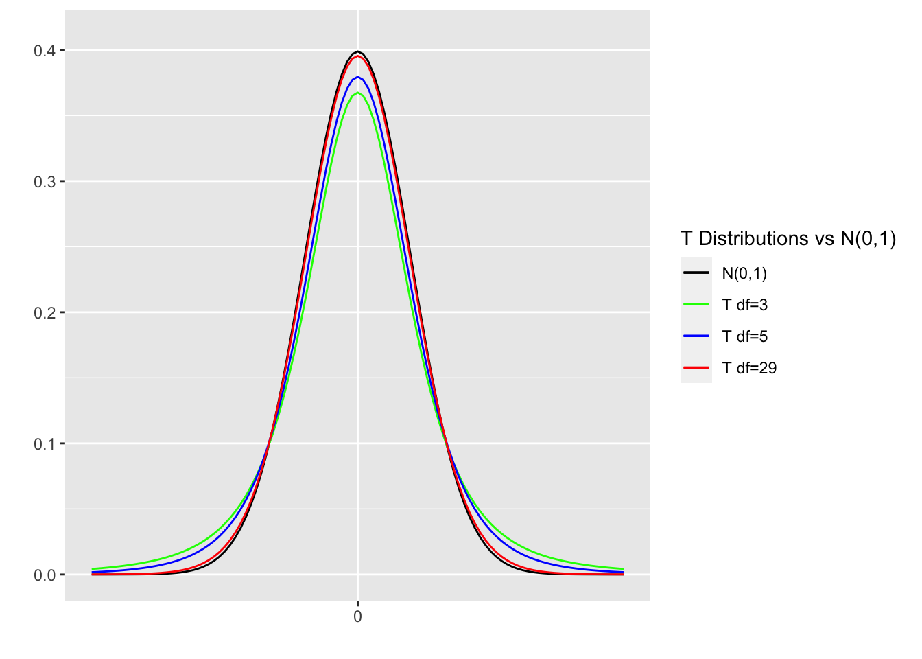
Figure 4.5: T Distributions Comparison
T distributions are symmetric, have mean of 0, and are roughly normally shaped. In those respects, T distributions are quite similar to the standard normal N(0,1) distribution. But there is one important difference. T distributions have “fatter tails” in general than the standard normal distribution, meaning more probability density is pushed outward away from the center. As the degrees of freedom get larger \((df\rightarrow\infty)\), T distributions get closer to being standard normal \((T_{df}\rightarrow N(0,1))\). Observe that the red \(T_{29}\) distribution is hard to distinguish from the black N(0,1) distribution, although the \(T_{29}\) does have slightly fatter tails. Recall that \(n=30\) is the most frequently cited bare minimum for a sample size to be considered to be “not small.”
A T distribution confidence interval is derived in the same way that the Z distribution confidence interval was derived above using the gnarly inequalities. The only differences are the use of \(s\) (computed from the sample) and that the value \(t_{\frac{\alpha}{2}}\) is obtained from a \(T_{n-1}\) distribution (mathematically because \(s\) is substituted for the unknown \(\sigma\)). Assuming that \(\sigma\) is unknown, the mathematics behind Cls for means require the following assumptions to hold.
ASSUMPTIONS for CI for Mean
- The population is normal, or the sample size is sufficiently large (say \(n\ge\) 30) and the population can be assumed to be normal-ish (symmetric, with only one mode (hump), etc.).
Under these assumptions, the CI for an unknow population mean \(\mu\) is given below. The multiplier \(t_{\alpha/2}\) comes from a T distribution \(T_{n-1}\) with \(n-1\) degrees of freedom.
\[\mu\in\left[\bar{x}-t_{\frac{\alpha}{2}}\cdot \frac{s}{\sqrt{n}}\; , \; \bar{x}+t_{\frac{\alpha}{2}}\cdot \frac{s}{\sqrt{n}}\right]\]
In shorter form, that’s \(\left[\bar{x}-t_{\alpha/2}\cdot SE\; , \; \bar{x}+t_{\alpha/2}\cdot SE\right]\) where \(SE=\frac{s}{\sqrt{n}}\).
For an example, suppose a pharmaceutical company needs to ascertain the average virus load that’s still present after patients take an anti-viral drug. The particular virus rarely infects humans, so the company is only able to test the new drug on 25 patients. Suppose \(n=25\) sample has a mean of \(\bar{x}=32.55\) parts per million, with a sample standard deviation of \(s=5.36\). The goal is to construct a 95% CI for the mean viral load.
The only additional information needed to construct the CI is the value \(t_{\frac{\alpha}{2}}\), which needs to be obtained from a \(T_{24}\) distribution since the sample size is \(n=25\). That is accomplished in the exact same way as discussed in Section 4.1, except using the qt (quantile T) function instead of qnorm. The qt function requires the df of the T distribution. To visualize the .025 right tail-area referenced below, refer back to Figure 4.1 for 95%. The concept is the same for T distributions.
The 95% CI for the mean viral load is then easily computed using this multiplier and the formulas presented above.
Why does substituting \(s\) for \(\sigma\) result in a T distribution? The obvious answer is the mathematics, some of which were hinted at above but are beyond the scope of this discussion. But it’s instructive to consider the T distribution concept in the abstract. There’s more uncertainty when a sample statistic is substituted for a population parameter. That uncertainty is evident in the fatter tails of the T distribution - more probability density is distributed away from the expectation. Why do the tails get thinner for large df? The larger the sample size \(n\), the more the sample tends to represent the population, hence less probabilistic uncertainty, hence “smaller tails” of the \(T_{n-1}\) distribution. Why \(n-1\)? Simply reason that substuting \(s\) for \(\sigma\) takes away 1 degree of freedom from the \(n\) independent observations (the random sample of size \(n\)) from the population.
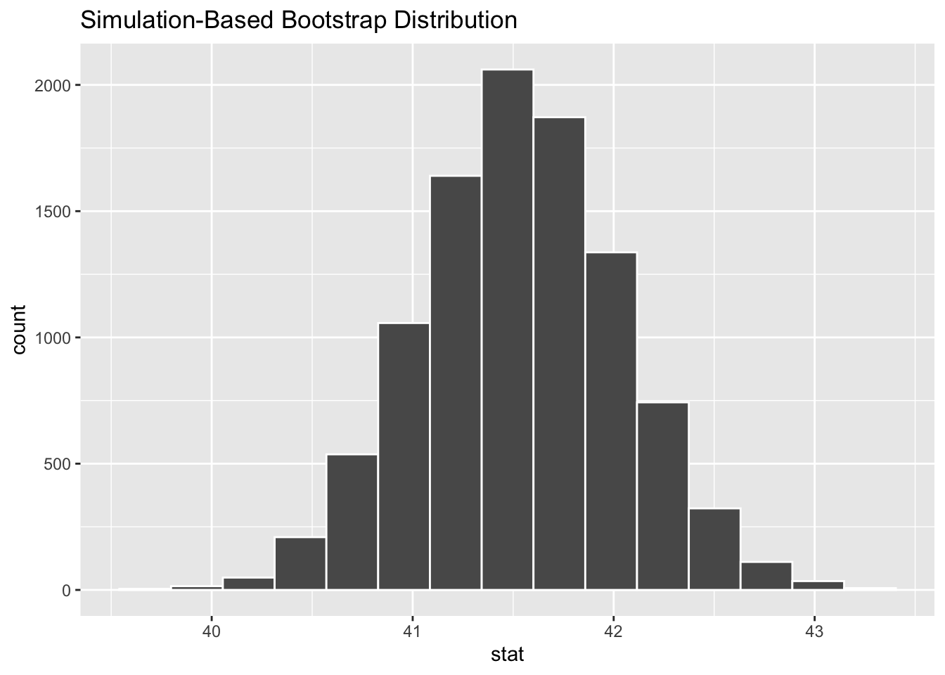
For an example using real data, we return to the data from the General Social Survey (GSS) that was loaded into a table named gss_survey in Section 4.2. That example featured the tvhours variable, but this time we’ll construct a 95% CI for the workhours variable that records how many hours the survey participants worked in the week prior to taking the survey. We’ll again filter the data to include only 2018, the most recent year featured in the data. The wrangling to compute the sample statistics and a histogram of the sample are shown below.
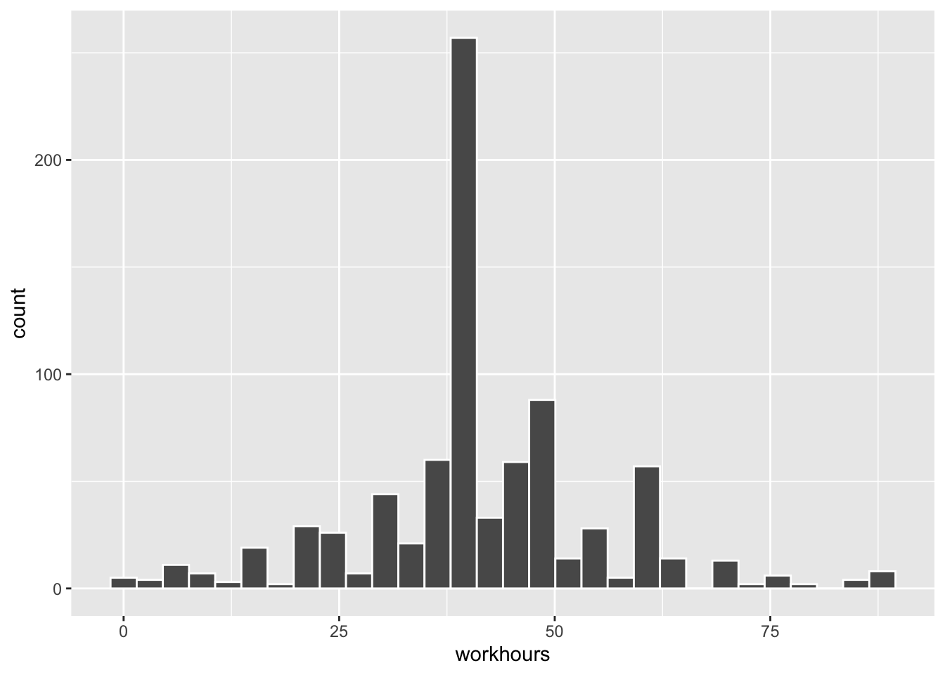
Here the sample size is \(n=828\) after removing a few NA values in the data. As in the previous example, the approximate sampling error will be computed as \(\frac{s}{\sqrt{n}}\). However, the value of \(t_{\frac{\alpha}{2}}\) as compute above for a 95% CI can NOT be used here since the sample size is different. This time it must be computed using a \(T_{827}\) distribution as shown below.
The 95% CI for the mean workhours is then easily calculated using this multiplier.
Some observations are in order. The 95% CI is roughly [40.5 42.5] and does not contain 40. So it can be inferred with 95% confidence that the unknown population mean \(\mu\) for hours worked is greater than 40. Based upon this survey data, it appears that people worked more than 40 hours, which is considered the standard work week in the USA.
We conclude this section with some information of historical curiosity that shines some light on the seemingly arbitrary \(n\le30\) criteria commonly stated for a sample being “small.” Most introductory statistics books cite that cutoff as if it’s some sort of magic number. Indeed, in most situations one would prefer a much larger sample size, which gives better normal approximations via the Central Limit theorem.
Under the assumption that the population being sampled is approximately normal, the mathematics behind the \(s\) for \(\sigma\) substitution ALWAYS results in a T distribution. However, a legacy from the pre-computing era is still found in many introductory statistics text books. Each potential sample size n results in a distinct \(T_{n-1}\) distribution. That’s an infinite number of different T distributions. Pre-computing stats books typically contain look-up tables in the appendices for finding \(t_{\frac{\alpha}{2}}\) values. But obviously an infinite number of look-up tables can’t be provided to cover all different T distributions. The most common solution was to provide T distribution look-up tables for about \(n\le30\).
But there is only one standard normal \(N(0,1)\) distribution, so one look-up table could provide \(z_{\frac{\alpha}{2}}\) values for commonly used confidence levels (\(1-\alpha\)). The rule of thumb was then if \(n>30\), it was ok to use the \(z_{\frac{\alpha}{2}}\) look-up table, even if what you technically needed to calculate was \(t_{\frac{\alpha}{2}}\).
In the example just above for \(n=828\), \(t_{\frac{.05}{2}}=1.9628\) (95% CI) was computed from a \(T_{827}\) distribution. The value for a 95% CI as shown in Figure 4.1 for a \(N(0,1)\) distribution is 1.959964 (rounded off to 1.96). So for \(n=828\), the difference is only about 0.003. After rounding, you get essentially the same CI using either value. However, even for a sample size of \(n=100\) which is considered relatively large for inference about means, the difference (between \(t_{\frac{\alpha}{2}}\) and \(z_{\frac{\alpha}{2}}\)) for a 95% CI is calculated below.
# T distribution look-up vs Z distribution look-up
qt(.975, df=99) - qnorm(.975, mean=0, sd=1)
## [1] 0.0243
For means estimations with low precision (like 41.5 in the above example), that difference still wouldn’t pose an accuracy problem. However, for more precise estimates, it could. As you have seen above, it’s equally easy using R’s q-* quantile distribution functions. So the bottom line is that, even though looking up Z values instead of T values is still prevalent in many stats books, in the modern computing era there is no reason not to use the more accurate T look-up when \(n\gt30\). Indeed, that’s what the mathematics say is appropriate and the \(n=30\) cutoff is, at least in part, an artifact from the pre-computing era.
4.4 Difference of Proportions
Before getting into the details, it’s instructive to begin with an example that shows the nature of a “difference of” CI. Consider again the gss_data data from the General Social Survey (GSS) that was used to demonstrate Cls for proportions in Section 4.2. That example derived a CI for the proportion of 2018 survey participants that are couch potatoes, an arbitrary notion we defined to be \(tvhours >= 3\) - relatively high TV watching per week.
There is a status variable in the gss_data that records marital status (married, divorced, etc). A 95% difference of proportions CI can be constructed from the data for the proportion of couch potatoes among married survey participants compared to the proportion of non-married potatoes. Such a CI is centered on the observed difference of proportions \(\widehat{p_1} - \widehat{p_2}\) between married (\(\widehat{p_1}\)) and non-married (\(\widehat{p_2}\)) survey participants to infer about the unknown population difference \((p_1-p_2)\).
The resulting 95% CI is [.028 , .156]. This CI will be computed below, but for now focus on the implications. Based on the survey, we are 95% confident that [.028 , .156] contains the unknown population difference \((p_1-p_2)\). Notice that 0 is NOT in the CI, which is entirely positive. That means we are 95% confident that \((p_1-p_2)>0\), from which the conclusion is that \((p_1>p_2)\). Thus, based on the survey data we are 95% confident that there are more non-married couch potatoes than married ones.
It would be tempting to construct a separate single-sample CI for each married and non-married category using the formulas from Section 4.2. If those two confidence intervals don’t overlap, that would indicate that the one of the proportions is larger than the other. But the probabilistic model for comparing “difference of” quantities like proportions and means is more robust when a single combined sampling distribution is used to simultaneously combine the sampling error from both samples - sort of a weighted average of the sampling variations from each sample. The resulting CI simultaneously factors in the sampling errors from each sample. That will become apparent from the formula for a “difference of” type of CI.
The general notation for a differences of proportions CI is as follows. Samples of sizes \(n_1\) and \(n_2\) are taken from each of two independent populations, and proportions \(\widehat{p_1}\) and \(\widehat{p_2}\) are calculated from the samples in order to infer about the unknown population proportions \(p_1\) and \(p_2\). As with Cls for single proportions, the \(\widehat{p_1}\) and \(\widehat{p_2}\) values computed from the samples are substituted into the mathematical formulas for the unknown population parameters \(p_1\) and \(p_2\), and the sampling distribution is approximately normal under the appropriate assumptions.
ASSUMPTIONS: Difference of Proportions CI
- Both sample sizes \(n_1\) and \(n_2\) are sufficiently large, and both \(\widehat{p_1}\) and \(\widehat{p_2}\) are not close to 0 or 1. Satisfying the \(np\gt 10\) and \(n(1-p) \gt 10\) criteria for EACH of \(\widehat{p_1}\) and \(\widehat{p_2}\) is usually sufficient unless \(\widehat{p_1}\) or \(\widehat{p_2}\) is close to 0 or 1, in which case even larger \(n_1\) or \(n_2\) is desirable.
- The populations are independent.
Then the CI for the unknown difference of population proportions \(p_1 - p_2\) is as given below.
\[ \small{ (p_1-p_2) \in \left[(\widehat{p_1} - \widehat{p_2}) - z_{\alpha/2}\sqrt{\frac{\widehat{p_1}(1-\widehat{p_1})}{n_1} + \frac{\widehat{p_2}(1-\widehat{p_2})}{n_2}} \;\;\;\; , \;\; \;\; (\widehat{p_1} - \widehat{p_2}) + z_{\alpha/2}\sqrt{\frac{\widehat{p_1}(1-\widehat{p_1})}{n_1} + \frac{\widehat{p_2}(1-\widehat{p_2})}{n_2}}\;\;\right] } \]
Yikes! That looks complicated, but perhaps not as much as the first impression. First, this says that the unknown difference of proportions \((p_1-p_2)\) is in an interval centered around the observed difference of proportions \((\widehat{p_1} - \widehat{p_2})\). The square root expression is essentially the estimated sampling error SE of the combined sampling distribution. Notice that it combines the sampling error from each of the independent distributions being sampled. The endpoints of the above CI can be simplified as simply \((\widehat{p_1} - \widehat{p_2}) \pm z_{\alpha/2} \cdot SE\). See, that’s not so bad.
Now recall the difference of proportions 95% CI that was discussed in concept at the beginning of this section for the proportion of General Social Survey (GSS) married survey participants that are couch potatoes compared to the proportion of non-married ones. The data wrangling is essentially the same as in Section 4.2, just with the addition of more filter criteria to create two different samples for married vs non-married.
gss_survey %>%
  filter(year == "2018" & status == "Married") %>%
  drop_na(tvhours,status) %>%
  summarize(
    married_potatoes = sum(tvhours >= 3),
    n1 = n(),
    p_hat1 = married_potatoes/n1   # proportion of couch potatoes
  )
## # A tibble: 1 × 3
##   married_potatoes    n1 p_hat1
##              <int> <int>  <dbl>
## 1              114   392  0.291
Notice above that drop_na(tvhours,status) removes a survey record if either the tvhours or status value is NA. You shouldn’t just do drop_na(), which would remove a survey record if ANY of the variables in that record are NA, which could remove some records for which both tvhours and status are actually valid.
There are several categories that are non-married status, so status != "Married" as used in the filter below catches them all.
gss_survey %>%
  filter(year == "2018" & status != "Married") %>%
  drop_na(tvhours,status) %>%
  summarize(
    non_married_potatoes = sum(tvhours >= 3),
    n2 = n(),
    p_hat2 = non_married_potatoes/n2   # proportion of couch potatoes
  )
## # A tibble: 1 × 3
##   non_married_potatoes    n2 p_hat2
##                  <int> <int>  <dbl>
## 1                  169   441  0.383
First note that the two sample sizes are different. That’s fine since the mathematics don’t require them to be the same. Also, it seems intuitive that the difference between the two sample proportions \(.38-.29=.09\) (or 9%) will end up being statistically significant. But that’s not known until the CI is computed and we can see whether it contains 0. The 95% CI is computed below using the the sample stats just computed above and the large formula for the difference of proportions CI.
# Combined Sampling Error
SE <- sqrt((.291*(1-.291))/392 + (.383*(1-.383))/441)
# Multiplier for 95% CI
z_alpha2 = 1.96
# CI
c((.291-.383) - z_alpha2*SE , (.291-.383) + z_alpha2*SE)
## [1] -0.1559 -0.0281
Since the CI does not contain 0, the conclusion is that the difference in proportions of the unknown population proportions is negative. That is, with 95% confidence, a smaller proportion \({p_1}\) of married people are couch potatoes than the proportion \({p_2}\) of non-married people.
The left endpoint of a such a CI is always negative when \(\widehat{p_1}\) is smaller than \(\widehat{p_2}\) since that makes the expression \((\widehat{p_1} - \widehat{p_2})\) negative. Alternately, the CI could instead be centered around \((\widehat{p_2} - \widehat{p_1})\) and the same conclusion would be reached. That is, the choice of which population to use for \(\widehat{p_1}\) vs \(\widehat{p_2}\) is somewhat arbitrary. The SE doesn’t change since switching the order of the sum under the square root doesn’t change anything (addition is commutative).
Reversing the roles of \(\widehat{p_1}\) and \(\widehat{p_2}\) as shown below in the CI endpoints calculation simply flips the CI to be positive, and results in the exactly same conclusion in the difference of proportions inference. The positive CI calculated below was used at the beginning of this section. The positive CI was less messy and perhaps easier to draw conclusions from for the sake of discussion than its negative counterpart.
# Reversing the order of the sample proportions doesn't change the conclusion.
c((.383-.291) - z_alpha2*SE , (.383-.291) + z_alpha2*SE)    # 95% CI
## [1] 0.0281 0.1559
Some remarks are in order about the assumptions necessary to make the mathematics behind the formulas valid. First, the \(np\gt 10\) and \(n(1-p) \gt 10\) criteria is easily satisfied for each of \(\widehat{p_1}\) and \(\widehat{p_2}\). But the requirement that the samples are independent is much less clear. In a survey or poll, for example, subdividing records using a categorical variable (married/non-married, male/female, …) results in independent samples. The data from one survey respondent is independent from another respondent. GSS could have conducted separate surveys for randomly selected married and non-married people. It doesn’t matter if that data were kept in separate tables, or combined into a single table using a categorical status variable as in the examples above. Either way, the two samples are considered independent.
For an example where the samples would not be independent, consider the tvhours and workhours variables. Each pair of such values in one row of data is collected from the same survey participant. The amount of workhours a person logs could easily affect their time left for tvhours (or unfortunately vise versa). Those two observations are dependent. Similarly, taking before and after measurements over some period of time on plants would result in dependent samples. How the plant grew prior to the before measurement could easily affect subsequent after measurements. In these cases, “difference of” tests would not be appropriate. Actually, in each of the dependent sample cases discussed just above, a single sample test would be appropriate. For example, calculating the quantity (change = after - before) would result in a single sample of change numbers. A single sample CI could then be easily constructed to infer about the average change in the population of the time period.
4.5 Difference of Means
This section begins with an example to illuminate the nature of a difference of means test. Suppose two different hybrid seeds are being tested to see which one results in taller plants. Samples of each seed are planted and carefully grown under the exact same conditions. Suppose hybrid1 reached an average height of \(\overline{x_1}=75.21\) cm and hybrid2 reached an average height of \(\overline{x_2}=74.89\) cm. Someone not versed in statistics might claim that hybrid1 grows taller on average than hybrid2. But is the difference actually statistically significant once sampling variation is taken into consideration?
Suppose a 95% confidence interval centered on the difference of means \((\overline{x_1}-\overline{x_2})\) is calculated to be [-0.0898,0.7298]. Notice that the CI contains 0. That is, when the point estimate \((\overline{x_1}-\overline{x_2})\) is expanded to an interval to account for sampling variation, 0 is a distinct possibility. Thus, the 95% CI includes the possibility that \((\mu_1-\mu_2)=0\), which would indicate the unknown population parameters could be equal. Based upon the samples, it’s not conclusive that the two hybrids produce different results.
The notation for a differences of means scenario is the same as with one mean, just expanded to two samples. In order to infer about two different independent populations, samples of sizes \(n_1\) and \(n_2\) are taken from each. The sample means are denoted by \(\overline{x_1}\) and \(\overline{x_2}\), and the standard deviations are denoted by \(s_1\) and \(s_2\). These point estimates are used to infer about the unknown population means \(\mu_1\) and \(\mu_1\).
In the unlikely case that there are reasonable estimates for the unknown population standard deviations \(\sigma_1\) and \(\sigma_1\), the mathematics point to constructing a CI for the difference of means using a Z distribution as shown in Section 4.1. With estimates for \(\sigma_1\) and \(\sigma_1\), the combined sampling error estimation is \(SE = \sqrt{\frac{\sigma_1^2}{n_1}+\frac{\sigma_2^2}{n_2}}\). The CI for the difference of means would then be constructed using the combined SE and a Z distribution \(z_{\alpha/2}\) multiplier.
However, substituting \(s_1\) and \(s_2\) for unknown \(\sigma_1\) and \(\sigma_2\) poses more of a mathematical challenge than making such a substitution when dealing with a single-sample CI. Several possibilities must be taken into consideration. Although \(\sigma_1\) and \(\sigma_2\) are unknown, it’s possible that \(\sigma_1 \approx\sigma_2\) (they are approximately equal) or \(\sigma_1/\sigma_2=K\) for some constant (they are proportional), or perhaps \(\sigma_1\) are \(\sigma_2\) not related in any way. The latter two cases are less applicable to situations that are commonly encountered in the practice of statistics, so we’ll defer discussion of those cases to a more advanced textbook.
The most common assumption in a difference of means analysis is that \(\sigma_1 \approx\sigma_2\), even though they are unknown. That’s actually a very reasonable assumption in many statistical applications. In quality control for manufacturing, different machines often produce slightly different results on average, but with very similar variability. In fact, if one machine’s output is less consistent (high variability) in its output, that may indicate a mechanical problem. Similarly, in drug and pharmaceutical testing, when one drug or medical device produces inconsistent results with significantly more variability than similar drugs or devices, that may be a sign that the product should be sent back to the research and development department to be rethought. Another way to rationalize the \(\sigma_1 \approx\sigma_2\) assumption is to consider why a difference of means analysis is being done in the first place - to see if similar populations are indeed essentially the same, or whether the difference is statistically significant. In contrast, comparing populations with very different inherent variability is more like a mismatched comparison of apples to oranges.
Using the \(\sigma_1\approx\sigma_2\) assumption when they are unknown still necessitates substituting the observed \(s_1\) and \(s_2\) into the mathematical formulas. But what happens if \(s_1\) and \(s_2\) calculated from the samples are not close to being equal, which would seem to violate the underlying assumption? That’s a distinct possibility because of sampling variation, even if \(\sigma_1\approx\sigma_2\) is actually true for the populations. There are formal statistical tests to indicate whether \(s_1\) and \(s_2\) are “close enough” not to undermine the \(\sigma_1\approx\sigma_2\) assumption upon which the mathematics hinge. But that is well beyond the scope of this discussion.
Studies that sample heights of men and women in the USA usually result in something like \(\overline{x_1}=69\) inches (about 5 feet 9 inches) with \(s_1\) usually about 3 for men, and \(\overline{x_2}=64\) inches (about 5 feet 4 inches) and \(s_2\) usually around 2.5 for women. Such a difference ( 3 is 20% larger than 2.5) between \(s_1\) and \(s_2\) is easily tolerable for a difference of means test. But when the difference starts getting more like 50%, many statisticians would put the brakes on the \(\sigma_1\approx\sigma_2\) assumption and move to another method for constructing the CI.
The heights of men and women example also illustrates the point that sometimes you don’t need a formal statistical analysis to draw a conclusion. Some things are simply obvious to the casual observer. In particular, one doesn’t need a someone with a Ph.D in statistics to conclude from the above numbers that men are taller on average than women. If a difference of means 95% CI is constructed (using the formulas below) even using relatively small sample sizes of 30, the CI is approximately [3.5,6.5]. Even based upon those small-ish samples, there is 95% confidence the unknown population means \(\mu_1\) and \(\mu_1\) differ by about 3 to 6 inches. The CI is nowhere close to containing 0, which would be necessary indicate a likelihood that the population means are the same.
Assuming that \(\sigma_1\) and \(\sigma_2\) are unknown, with \(s_1\) and \(s_2\) substituted into the SE formula instead, the difference of means CI require the following assumptions to hold.
ASSUMPTIONS for Difference of Means CI:
- Both populations are normal, or both sample sizess \(n_1\) and \(n_2\) are sufficiently large (say \(\ge\) 30), and both populations can be assumed to be normal-ish (symmetric, with only one mode (hump), etc.).
- The populations have approximately the same standard deviation. Because of sampling variation, the observed \(s_1\) and \(s_2\) will likely differ, but ideally not by much.
- The populations are independent.
Under these assumptions, the CI for unknown \((\mu_1-\mu_2)\) is given below. The multiplier \(t_{\alpha/2}\) comes from a \(T_{n_1+n_2-2}\) distribution with \(n_1+n_2-2\) degrees of freedom.
\[ (\mu_1-\mu_2) \in \left[ \; (\overline{x_1}-\overline{x_2}) - t_{\alpha/2}\cdot S_p^2 \cdot \sqrt{\frac{1}{n_1}+\frac{1}{n_2}} \;\;\;\; , \;\; \;\; (\overline{x_1}-\overline{x_2}) + t_{\alpha/2} \cdot S_p^2 \cdot \sqrt{\frac{1}{n_1}+\frac{1}{n_2}} \;\;\;\right] \]
Above, \(S_p^2\) is called the pooled variance, a type of weighted average of the sampling variations from the two independent samples. It can be computed directly from the samples as shown below.
\[ S_p^2 = \sqrt{\frac{(n_1-1)s_1^2 + (n_2-1)s_2^2}{n_1+n_2-2}} \]
Again, this seems quite complicated until you back away from the details. The endpoints of the CI are of a form that should be familiar to you by now: \((\bar{x_1}-\bar{x_2}) \pm t_{\alpha/2} \cdot SE\) where \(SE\) is the pooled variance \(S_p^2\) times the square root expression. In this context, the \(SE\) is essentially an elaborate weighted average that estimates the combined sampling error. It would be cleaner to consolidate the square root stuff into the \(S_p^2\) expression, but \(S_p^2\) is kept separate in the mathematical theorems as a matter of convenience.
Now back to the example from the beginning of this section of testing hybrid seeds to see which one grows taller plants. The difference of means CI was [-0.0898,0.7298] and since it contains 0, the conclusion was that the samples didn’t provide sufficient evidence that the two hybrids produce different results. Although the two samples had different means, that difference wasn’t statistically significant. The sample statistics and calculations behind that example are shown below.
# Hybrid 1 Sample
n1 <- 40
x1 <- 75.21
s1 <- .89
# Hybrid 2 Sample
n2 <- 40
x2 <- 74.89
s2 <- .95

# Sampling Error
pooled_variance <- sqrt(((n1-1)*s1*s1 + (n2-1)*s2*s2)/(n1+n2-2))
SE <- pooled_variance * sqrt(1/n1 + 1/n2)

# Multiplier for 95% CI
t_alpha2 <- qt(.975, df=78)   # 78 = 40 + 40 - 2

# CI
c((x1-x2) - t_alpha2*SE , (x1-x2) + t_alpha2*SE)
## [1] -0.0898  0.7298
You may have noticed that the above example presents statistics computed from samples, but doesn’t provide the actual sample data. This chapter has imported and processed data in several examples, so there was nothing new to be gained from that in this section. Indeed, the focus here is to highlight the assumptions and formulas associated with a difference of means CI.
4.6 Bootstrap Distributions
The key ingredient in Bootstrapping is sampling with replacement. It’s best to proceed by example. The following code creates a simple table containing a virtual box of balls numbered 1,2,….,10. It then calls the slice_sample() function twice, each time randomly sampling 5 balls with replacement from the virtual box of 10 balls. That means draw one ball, record the number, put it back in the box, draw another ball, put it back in the box, and so forth. The slice_sample() function defaults to replace=FALSE as it was used in Section 3.3 to sample from the dragon population without replacement. Below replace=TRUE overrides the default to sample with replacement.
box_of_balls <- tibble(
  balls = 1:10
)
box_of_balls
sample_with_replace1 <- slice_sample(box_of_balls, n=5, replace=TRUE)
sample_with_replace2 <- slice_sample(box_of_balls, n=5, replace=TRUE)
The output of the above code is shown below with the “box” of balls on the left, and the two with replacement samples on the right. Observe the effect of sampling with replacement. Since the ball is replaced after each draw, the same ball often ends up being drawn multiple times. This seems like a very strange way to do sampling, but it very interesting applications in statistical simulations.
| box_of_balls |
|---|
| 1 |
| 2 |
| 3 |
| 4 |
| 5 |
| 6 |
| 7 |
| 8 |
| 9 |
| 10 |
| sample_with_replace1 |
|---|
| 2 |
| 9 |
| 9 |
| 9 |
| 5 |
| sample_with_replace2 |
|---|
| 7 |
| 7 |
| 3 |
| 3 |
| 6 |
To demonstrate a very cool application of sampling with replacement, we’ll return to the “real” data on dragon wingspans from Section 3.3 where a sample of \(n=75\) dragon wingspans was taken from a known population of dragons. That example will again be helpful here because knowing the population parameters allows us to assess how accurate inferences about the population made from the random sample actually are.
For a refresher on the dragon_sample, a histogram of the exact same \(n=75\) sample that was used in Section 3.3 is shown below, together with typical sample stats computed from it.
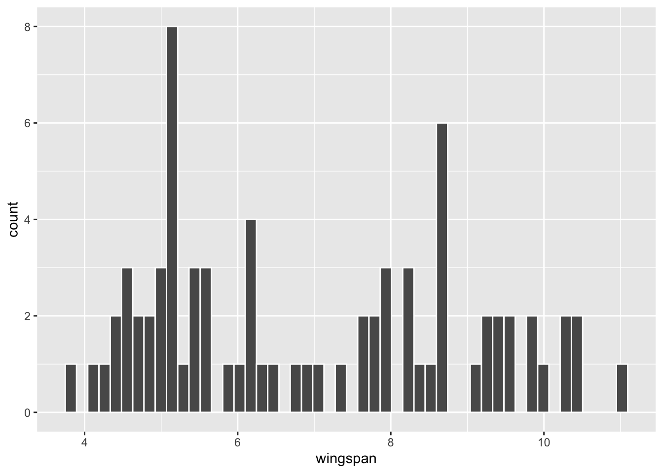
| sample_mean | sample_sd | n |
|---|---|---|
| 6.96 | 2 | 75 |
Now, well use the rep_slice_sample() (repetitive slice sampling) function that’s provided by the Infer package. Recall that rep_slice_sample() was introduced in Section 3.3 to sample repetitively from the dragon population to demonstrate the Central Limit Theorem by computer simulation. But this time, the samples are actually re-samples of size 75 from the original size \(n=75\) dragon sample. Think about that for a second: the re-samples are taken from the sample (not the population) and are the exact same size as the sample. Without replacement that would accomplish nothing because each re-sample would be exactly the same as the original sample. However, when the re-samples are taken with replacement, each re-sample tends to be slightly different from the original.
The code below takes 10,000 distinct re-samples with - with replacement - from the original n=75 sample, each re-sample being the same size as the original. Notice that replace=TRUE is added to the rep_slice_sample() function call to override the default. The result is the bootstrap_resamples table which has 750,000 rows, organized by the replicate numbers that keep track of the 10,000 distinct re-samples. The standard R view of the table only shows the first few wingspans from replicate #1.
library(infer) # contains rep_slice_sample() function
# 10,000 re-samples WITH replacement
bootstrap_resamples <- dragon_sample %>%
  rep_slice_sample(n=75 , reps=10000 ,  replace=TRUE)
bootstrap_resamples
## # A tibble: 750,000 × 2
## # Groups:   replicate [10,000]
##    replicate wingspan
##        <int>    <dbl>
##  1         1      8.6
##  2         1      8.6
##  3         1      7.6
##  4         1      5
##  5         1      8.3
##  6         1      9.4
##  7         1      9.4
##  8         1      4.6
##  9         1      5.1
## 10         1      8.6
## # ℹ 749,990 more rows
The code below groups the bootstrap_resamples by the replicate numbers in order to compute a separate mean for each of those 10,000 re-samples. The result is the bootstrap_distribution_of_means table, only the first few rows of which are shown. It has 10,000 rows, each containing the mean of one of the re-samples.
# Calculate a separate mean for each of the 10,000 re-samples
bootstrap_distribution_of_means <- bootstrap_resamples %>%
  group_by(replicate) %>%
  summarize(resample_mean = mean(wingspan))
bootstrap_distribution_of_means
## # A tibble: 10,000 × 2
##    replicate resample_mean
##        <int>         <dbl>
##  1         1          7.27
##  2         2          6.89
##  3         3          6.71
##  4         4          6.98
##  5         5          6.98
##  6         6          6.99
##  7         7          7.48
##  8         8          6.49
##  9         9          6.98
## 10        10          6.91
## # ℹ 9,990 more rows
It’s important to stop and reflect upon the bootstrap_distribution_of_means table. Because of sampling with replacement, some dragons from the original sample might be included twice, or even more, in a re-sample. Other dragons from the original sample might not even be included in a re-sample. Therefore, each re-sample tends to have a different mean as you can see in the bootstrap_distribution_of_means table. In essence, each re-sample is kind of a “phantom sample” or “tweaked sample” that bears some resemblance to the original sample in that all members of the re-sample are drawn from the original sample, but yet the re-sample is subtly different.
Effectively, the re-samples from the sample induce sampling variation, thereby simulating the sampling variation that would be inherent when sampling from the population. In other words, each re-sample simulates the act of taking a different original random sample from the population. It follows that a very large number of such re-samples, say 10,000, should model the \(n=75\) sampling distribution.
The code below produces the histogram on the right side of Figure 4.6. It shows the distribution of the 10,000 bootstrap_distribution_of_means computed above. The two plots on the left side of Figure 4.6 show similar bootstrap distributions of re-sampled means, just using fewer repetitions.
# Histogram of Bootstrap Distribution for the 10,000 bootstrap_distribution_of_means
bootstrap_distribution_of_means %>%
  ggplot(aes(x = resample_mean)) +
  geom_histogram(bins = 30, color = "white") +
  labs(x = "Bootstrap Sample Means")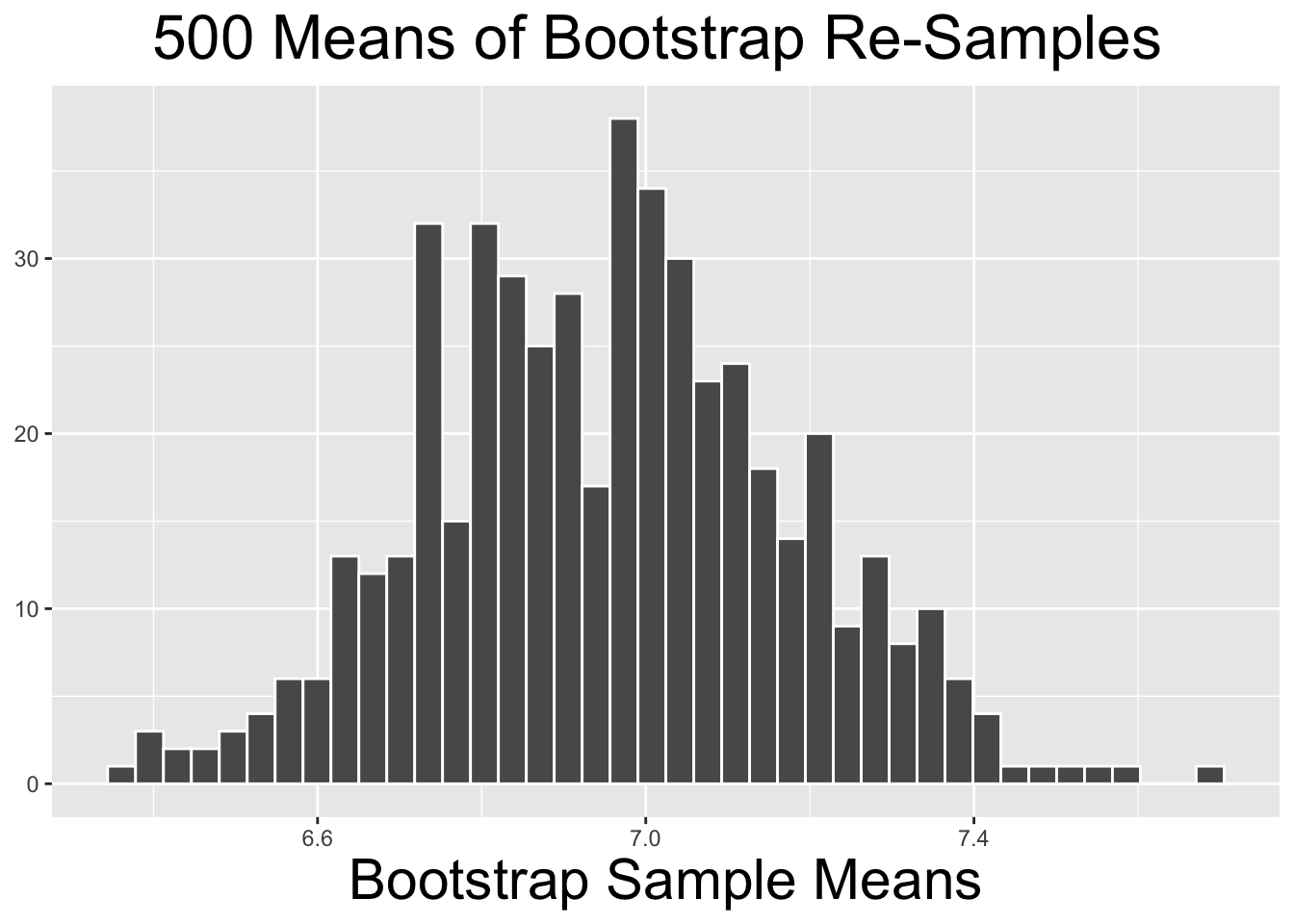
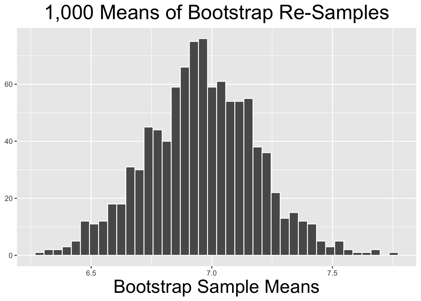
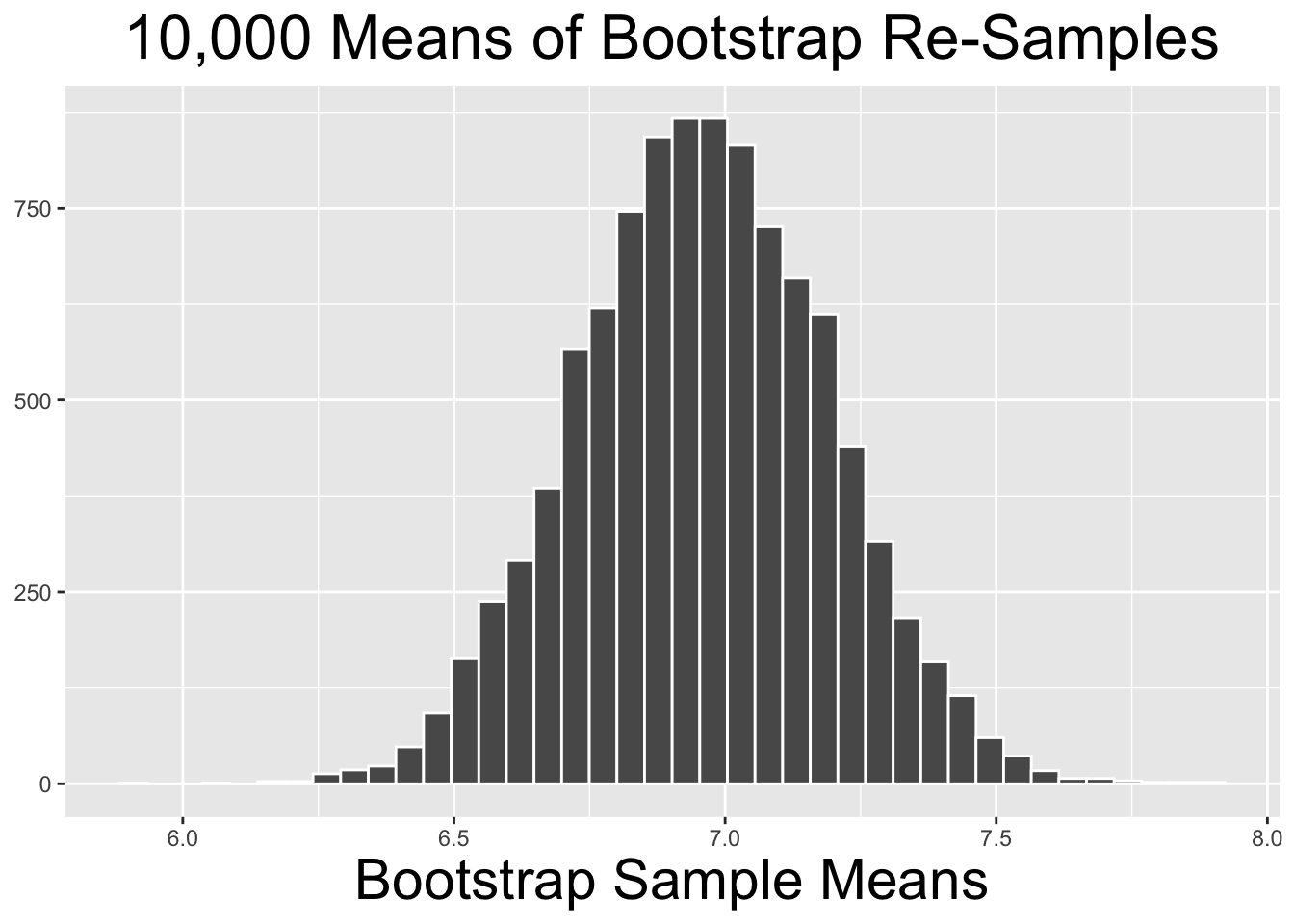
Figure 4.6: Bootstrap Distributions for Different Numbers of Repetitions
The two bootstrap distributions on the left of Figure 4.6 obviously appear less normal than the one on the right. As a general principle, the more re-sample repetitions that go into a bootstrap distribution, the more normal the bootstrap distribution tends to be. Less bootstrap repetitions tend to be needed if the original sample is normal-ish. In general, 10,000 repetitions is usually adequate and easily doable with typical desktop computing power. In some situations - a very large original sample for example - it can be desirable to do 100,000, a million, or even more repetitions. But it may require more than typical computing power to run such large numbers of repetitions relatively quickly.
Having explained the basic concepts through examples, it’s instructive to formally define the terminology pertinent to bootstrap distributions.
Bootstrap Terminology
Given an original sample of size \(n\), a bootstrap sample is a re-sample with replacement of size \(n\) from the original sample. A sample statistic, such as a mean, computed from a bootstrap sample is likely somewhat different from that of the original sample. When multiple bootstrap samples are taken, the resulting collection of bootstrap sample statistics is called a bootstrap distribution. A bootstrap distribution is a simulated sampling distribution constructed solely from the original sample. The mean and standard deviation of a bootstrap distribution are examples of bootstrap statistics - descriptive statics of the bootstrap distribution.
Having computed the bootstrap_distribution_of_means above for 10,000 bootstrap samples, it’s a simple matter to compute the bootstrap statistics that describe the bootstrap distribution.
# Calculate the Bootstrap Statistics
bootstrap_distribution_of_means %>%
  summarize(
      bootstrap_distribution_mean = mean(resample_mean),
      bootstrap_distribution_SE = sd(resample_mean)
  )
## # A tibble: 1 × 2
##   bootstrap_distribution_mean bootstrap_distribution_SE
##                         <dbl>                     <dbl>
## 1                        6.96                     0.231
It is important to understand that the bootstrap statistics computed above are the mean and standard deviation of the 10,000 repetition bootstrap distribution shown on the right side of Figure 4.6. The bootstrap distribution mean of 6.96 is exactly the same as the mean of the original sample. In general, the mean of the original sample is the expectation for the mean of a bootstrap distribution. That makes sense since each of the bootstrap samples is a “tweak” of the original sample.
The bootstrap distribution standard deviation of .231 is very close to the \(SE=.257\) of the sampling distribution that was computed using the Central Limit Theorem in Section 3.4. Since each bootstrap sample simulates the act of taking a different original random sample from the population, it makes sense that the bootstrap distribution standard deviation is close to the sampling distribution SE.
The procedure outlined above is often simply called Bootstrapping and is summarized below.
Bootstrapping Procedure:
- Take an original random sample of size \(n\) from the population.
- Compute a bootstrap distribution by calculating a sample statistic (mean, proportion, etc) separately from each of many bootstrap samples taken repetitively from the original sample.
- The bootstrap distribution will be approximately normal for a large enough number of repetitions, say 10,000.
- The standard deviation of the bootstrap distribution - a bootstrap statistic - is a simulated estimate for the SE of the size \(n\) sampling distribution.
4.7 Bootstrap Confidence Intervals
One of the main applications of bootstrapping is for computing confidence intervals. This section explores two methods for constructing a CI from a bootstrap distribution: the Standard Error (SE) Method and the Percentile method. We’ll begin with the SE method.
Bootstrap Standard Error (SE) Method
The SE estimate for the CI is the standard deviation of the bootstrap distribution. The CI centered on the sample mean \(\bar{x}\) is constructed as usual, with endpoints \(\bar{x} \pm z_{\alpha/2} \cdot SE\). This assumes that the bootstrap distribution is approximately normal with minimal skew.
For an example, we’ll continue with the 10,000 repetition bootstrap_distribution_of_means table that was computed in the previous section. The distribution of those bootstrap sample means is shown on the right of Figure 4.6, and the standard deviation bootstrap statistic was computed to be \(SE=.231\). As discussed in the previous section, the bootstrap SE is a computational estimate of the sampling error for samples of size \(n=75\). The resulting 95% bootstrap CI centered on the observed sample mean \(\bar{x}=6.96\) is calculated below using the \(z_{\alpha/2}=1.96\) multiplier from the standard normal distribution.
# 95% CI using bootstrap distribution SE
SE <- .231
z_alpha2 <- 1.96   # 95% CI
c(6.96 - z_alpha2*SE, 6.96 + z_alpha2*SE)
## [1] 6.51 7.41
Now for the bootstrap Percentile method. After the definition, we’ll proceed with with the same example for the sake of comparison.
Bootstrap Percentile Method
The endpoints of the CI are percentiles calculated from the bootstrap distribution. The percentiles are determined by the total tail area \(\alpha\). This does not require the bootstrap distribution to be approximately normal. If it is skewed, the CI may not be exactly centered on the sample mean \(\bar{x}\),
For example, the total of both tail areas for a 95% CI is 5%. So the lower endpoint of the percentile method CI is the 2.5th percentile, and the upper endpoint is the 97.5th percentile. That is, if all 10,000 numbers in the bootstrap_distribution_of_means table are sorted in increasing order, the 2.5th percentile is approximately the 250th number and the 97.5th percentile is approximately the 9,750th one. That’s easily computed using the quantile() function as shown below. The calculation could also have been done using two separate function calls like quantile(data, .025), but sending both percentiles to the function as a vector gets the job done with only one function call.
The first few sections in this chapter presented theory-based confidence intervals derived using mathematics and the Central Limit Theorem. This section has introduced simulation-based confidence intervals using computational bootstrapping. Before moving on, it’s worth stepping back from the details for a general comparison. A 95% CI is used below for the sake of discussion, but the idea applies to any confidence level.
Simulation-Based vs Theory-Based Confidence Intervals
Section 4.1 pointed out that a theory-based 95% CI is essentially the center 95% of the theoretical \(\mu\)-centered sampling distribution, but recentered around the sample mean \(\bar{x}\). In a bootstrap simulation, there is no theoretical \(\mu\)-centered sampling distribution, just a simulated \(\bar{x}\)-centered bootstrap distribution. A bootstrap CI is also the “center” 95% of the bootstrap distribution. The bootstrap SE and percentile methods just calculate the notion of “center” in different ways.
The bootstrapped Cls from each of the SE and Percentile methods are very similar, actually the same if rounded to two decimal places. For further comparison, we’ll compute the theory-based 95% CI derived from the Central Limit Theorem as shown in Section 4.3 using a T Distribution with 74 degrees of freedom. The calculation is shown below.
# Theory-based 95% CI using T distribution
s <- 2.0049          # from dragon sample
SE <- s/sqrt(75)     # CLT
t_alpha2 <- qt(.975, df=74)
c(6.96 - t_alpha2*SE, 6.96 + t_alpha2*SE)
## [1] 6.50 7.42
And finally, we might as well throw in the CI computed in Section 4.1 using the known population standard deviation \(\sigma\) in \(SE = \frac{\sigma}{\sqrt{n}}\) instead of substituting \(s\). All 4 Cls are shown below for comparison.
| Method | CI |
|---|---|
| Simulation-based Bootstrap SE | \([6.51,7.41]\) |
| Simulation-based Bootstrap Percentile | \([6.51,7.41]\) |
| Theory-based (substitute s for \(\sigma\)) | \([6.50,7.42]\) |
| Theory-based (know \(\sigma\)) | \([6.46,7.46]\) |
The Cls in the top three rows above are all calculated entirely using the dragon sample. However, the bottom row is calculated from a known population parameter, a luxury usually not available when doing inference. Thus, one might expect the bottom one to be somewhat different from the others since taking the sample involves sampling error. But the main takeaway from this is that the theory-based CI derived from Mathematics/CLT and the sample sd \(s\) is very similar to the simulation-based bootstrapped ones, within .01 in fact.
For an example involving real data, recall the tvhours_2018 sample from the GSS survey used previously in this chapter. We’ll compute a 99% bootstrap CI using each method presented above. The calculations to derive the bootstrap_distribution_of_proportions are shown below. The table contains 10,000 resample_proportion values, each being the proportion of couch potatoes in a re-sample. The only difference between the code below and that of the previous section is that 10,000 proportions are calculated instead of means.
# Bootstrap Distribution of 10,000 Proportions
bootstrap_distribution_of_proportions <- tvhours_2018 %>%
  rep_slice_sample(n=833 , reps=10000 ,  replace=TRUE) %>%
  group_by(replicate) %>%
  summarize(
    num_couch_potatoes = sum(tvhours >= 3),
    n = n(),
    resample_proportion = num_couch_potatoes/n   # proportion of couch potatoes
  )
# Bootstrap Statistics from the Bootstrap Distribution
bootstrap_distribution_of_proportions %>%
  summarize(
      boot_dist_mean = mean(resample_proportion),
      boot_dist_SE = sd(resample_proportion)
  )
The bootstrap statistics from the 2nd block of code above are shown below on the right. The code that creates the histogram of the bootstrap distribution on the left is not shown. Note that the boot_dist_mean is the average of the 10,000 proportions. It is almost exactly equal to the original sample proportion \(\hat{p}\) as is expected.
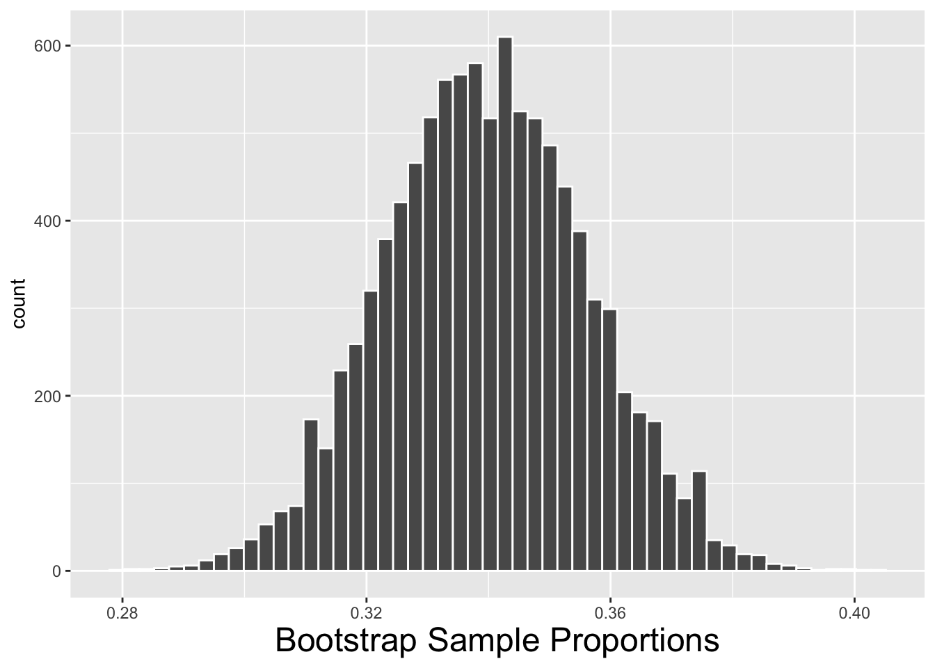
| boot_dist_mean | boot_dist_SE |
|---|---|
| 0.34 | 0.016 |
The calculation for the bootstrap SE method CI is shown below. Of course, the CI is centered on the observed sample proportion \(\hat{p}=.340\) and the SE bootstrap statistic was computed above from the bootstrap distribution.
# Bootstrap SE method 99% CI
SE <- .0164
z_alpha2 <- 2.58   # 2.58 = qnorm(.995, mean=0, sd=1)
c(.340 - z_alpha2*SE, .340 + z_alpha2*SE)
## [1] 0.298 0.382
The calculation for the bootstrap percentile method CI is shown below. The calculation is quite simple assuming that the correct .005 (left) and .995 (right) tail areas are used for a 99% CI.
# Bootstrap Percentile method 99% CI
quantile(bootstrap_distribution_of_proportions$resample_proportion, c(.005,.995))
##  0.5% 99.5%
## 0.298 0.383
The two bootstrap Cls are shown below, and for comparison so is the theory-based 99% CI that was calculated in Section 4.2. As you can see they are very, very close up to 3 decimal places. The .001 discrepancy in the right endpoint of the Bootstrap Percentile CI could easily be the result of rounding off some of the numbers used in the calculations or the way percentiles for finite samples are calculated.
| Method | CI |
|---|---|
| Simulation-based Bootstrap SE | \([.298,.382]\) |
| Simulation-based Bootstrap Percentile | \([.298,.383]\) |
| Theory-based (substitute \(\hat{p}\) for \(p\)) | \([.298,.382]\) |
Cls constructed by \(\pm\) a multiple of an SE estimate, either derived from bootstrapping or math, are always centered on the observed sample statistic (\(\hat{p}\), \(\bar{x}\), …). However, because of the way a Bootstrap Percentile CI is constructed, the sample statistic many not be exactly in the center of the CI. If the bootstrap distribution is roughly symmetric, then the sample statistic should be roughly in the center of the Bootstrap Percentile CI.
Observe the summary of the 10,000 bootstrap sample proportions below which shows that the mean and median of that bootstrap distribution are equal. That indicates that the bootstrap distribution is not skewed. Therefore it is no surprise that both bootstrap CI methods produced roughly the same result.
summary(bootstrap_distribution_of_proportions$resample_proportion)
##    Min. 1st Qu.  Median    Mean 3rd Qu.    Max.
##   0.279   0.329   0.340   0.340   0.351   0.403
Having done comparisons between the two bootstrap CI methods, and also comparing bootstrapping to the traditional theory-based methods, natural questions arise: Which is more accurate in general? Which method should I use in a given situation? The question of theory-based vs bootstrap is more tricky to answer, so we’ll defer that until the next section. But when bootstrapping, the question of percentile method is more easily answered. In fact, the discussion just above about symmetry of the bootstrap distribution gives a strong clue.
To further explore that, consider the example below of a sample that’s highly skewed. The distribution of this size \(n=25\) sample is shown below on the left, and a 10,000 repetition bootstrap distribution is shown on the right. The sample is highly skewed right: \(median=.260\), \(mean=.745\). It’s not obvious visually, but the bootstrap distribution is also skewed right: \(median=.736\), \(mean=.745\). The 10,000 re-sample bootstrap procedure has substantially lessened the skew, but it’s still there.
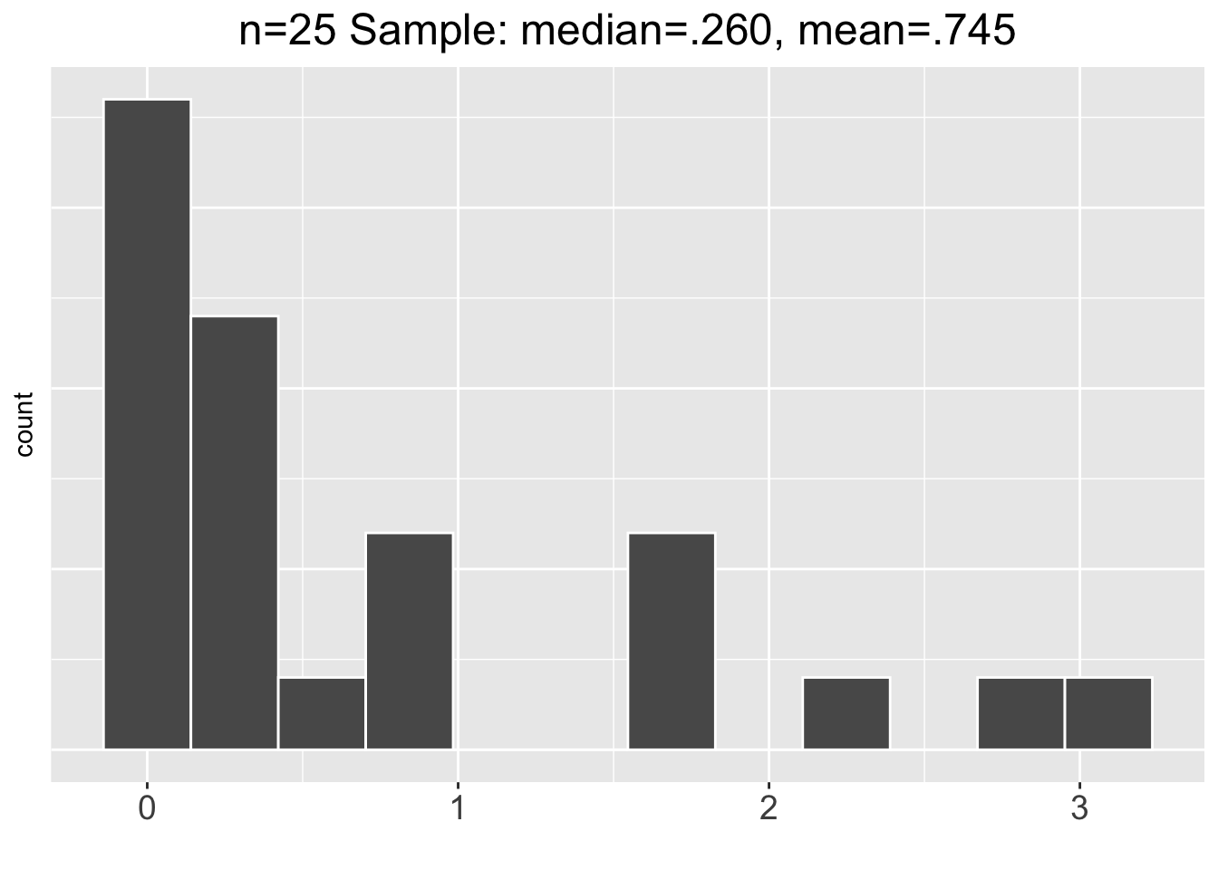
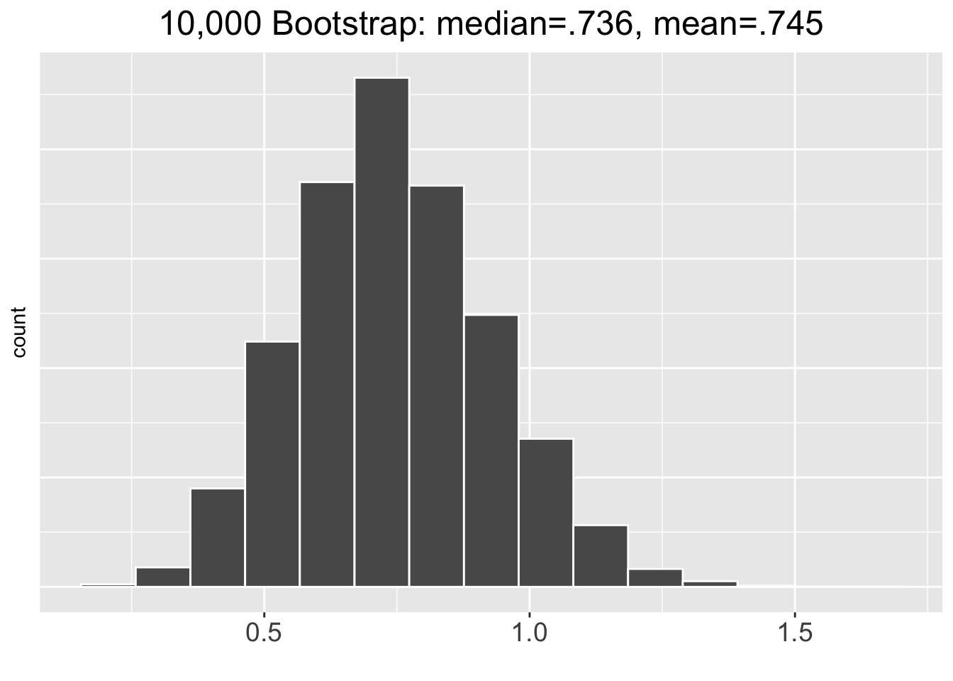
For the above skewed data, the bootstrap SE method 95% CI is \([.386,1.103]\) and the percentile method 95% CI is \([.403,1.120]\). Even though the skew of the bootstrap distribution seems minimal, the two bootstrap CI methods produce significantly different results. In situations with a highly skewed sample that results in a skewed bootstrap distribution, the bootstrap percentile method is generally considered to be more accurate. This is especially true when the sample size is small as in the previous example.
The curious reader may wonder whether doing 100,000 or even a million bootstrap re-samples would make any difference. In the \(n=25\) highly skewed sample discussed just above, upping the bootstrap repetitions to 100,000 results in changes on the order of magnitude of about .0001 which is outside the round off error. In this case, doing 1 million bootstrap repetitions offers no significant improvement, and takes several seconds to complete on a fast desktop computer.
In many situations, 10,000 bootstrap repetitions is enough. In a highly sensitive analysis with lots of decimal place accuracy required, one would ideally increase the number of bootstrap repetitions until the results stabilize at the desired accuracy. For example, if 4 decimal places of accuracy is desired and a 10,000 repetition bootstrap tends to give a different result in the 4th decimal place each time you run it, then try again with 100,000. Hopefully that stabilizes, giving the same result to 4 decimal places each time you run it. If not, up the repetitions again. But keep in mind that both the size of the sample being bootstrapped and the number of repetitions increase the computation time, which could become a limitation on a typical desktop computer in which case a more powerful computer system could be used.
4.8 Why Bootstrap?
The phrase to “pull yourself up by your bootstraps” has been commonly used in literature and colloquial conversations for centuries. It means that you improve your situation exclusively through your own efforts, without any other help. The bootstrap simulation procedure in statistics borrows from that notion in that the data is “pulling itself up by its own bootstrap.” Suppose you have a sample of data, with absolutely no other assumptions about the population from which the data was drawn. Without such assumptions, mathematical theory provides little or no help in inferring about population parameters. The bootstrap procedure, using ONLY the sample itself, allows you to infer about population parameters by simulating the sampling error inherent in random sampling. Bootstrap “tweaking” of the sample many thousands of times to obtain “alternate” samples simulates the theoretical concept of a probability model for the space of all possible samples of that size.
This chapter has presented both theory-based (math/CLT) and simulation-based (bootstrap) methods of inference. You may have noticed that the mathematics for the various types of Cls presented in this chapter depend on normality and other assumptions. In the world of theory-based inference, it’s all about assumptions, assumptions, assumptions.
It’s instructive to clarify this discussion by highlighting when theory-based Cls are not reliable. The theory-based mathematical Cls presented in this chapter are NOT valid for:
- Single proportion Cls when the sample size is small or \(\hat{p}\) is close to 0 or 1 (\(np\gt 10\) fails).
- Single mean Cls when the population is not normal-ish and sample size is small.
- Any “difference of” Cl when the samples aren’t totally independent.
- Difference of proportion Cls when the sample size is small or \(np\gt 10\) fails for either sample.
- Difference of means Cls when either population is not normal-ish, or either sample size is small, or the samples have significantly different standard deviations.
The above points are basically the logical negations of the required assumptions for theory-based Cls that were listed in the first few sections in this chapter. In some cases when the assumptions don’t hold and the theory-based CI presented in this chapter is not reliable, there are more advanced theory-based approaches that might work. Such topics are often covered in detail in advanced stats courses or even graduate school.
The mathematics for Non-Parametric inference are particularly gnarly. The mathematical theory for parameter estimation (mean, standard deviation, variance,…), is based on assumptions about an underlying probability distribution. In contrast, quantities such as medians and percentiles are called Order Statistics because they are based on a linear ordering of the sample, not a formula derived from a probability distribution model. The term Non-Parametric Statistics, also called distribution-free statistics, essentially refers to inference about such non-parameter order statistics. There are some theory-based techniques for non-parametric statistical analyses, but the situation is much more difficult since sampling error SE estimates are complicated, often being semi-reliable mathematical approximations themselves, or even impossible to calculate mathematically.
In applications such as non-parametric analyses, bootstrapping (and other simulation techniques) provide an alternative when mathematical theory isn’t sufficient. Even for a routine non-parametric analysis, like inferring about an unknown population median or quartile, bootstrapping may be the most appropriate option. But even bootstrapping has it’s limitations, being most reliable when inferring about a non-parametric value near the “middle” of a sample, rather than about extreme values near the “edges” of a sample.
The list below provides a quick overview summarizing important points about bootstrapping, including the points discussed just above and also things observed in the examples in the previous sections of this chapter. In short, no data scientists should be without Bootstrapping in their toolkit!
- When the assumptions hold and the theory-based approach to estimating the SE is robust, bootstrapping tends to give very similar results.
- When the data doesn’t fully satisfy the assumptions required by mathematics, the bootstrap simulation-based approach tends to give more reliable results.
- The traditional mathematical approaches for certain types of statistical inference, such as non-parametric analyses, tend to be less robust than those for parametric analyses. In some cases, sampling error estimates are problematic or impossible using mathematics. Simulation-based approaches like bootstrap may be the only viable option.
- Bootstrap sampling is used in various machine learning algorithms. In that context, the technique is called bootstrap aggregating, or simply bagging.
- The huge leap forward in computing power has made simulation-based techniques much more practical for the average person. (Some might argue that no statisticians are average people!) Even as recent as the year 2000, running complex simulation-based models with tens of thousands of iterations might be problematic without access to clusters or supercomputers.
- New tools such as the Infer package make it much easier to do simulation-based inference for people who are not experienced programmers.
The obvious question that arises from this discussion is the following:
Which inference method should be used in a given situation?
It’s not just a question of theory-based vs simulation-based, which may answer itself based upon whether the assumptions required for a theory-based inference are satisfied (or almost). This question often arises even when choosing between different theory-based approaches which abound in advanced statistical books and research papers. Even highly experienced statisticians may disagree upon which approach is best. Inferential statistics is about estimating things, which is rarely an exact science.
The answer to the question is often simply about convention - what’s accepted practice in a given research field. For example, social sciences (psychology, anthropology, …) may have somewhat less rigorous guidelines than medical and pharmaceutical sciences. In many cases, the question resolves to what statistical analysis is acceptable to peer-refereed science journals. In some cases, the answer to the question might be dictated by a bureaucratic or government agency. For example, a pharmaceutical company might submit a study to the US FDA (Food and Drug Agency) to seek approval for a new drug. The FDA Ph.D statisticians might request or demand an alternate statistical analysis be submitted for the sake of comparison. Those Ph.D statisticians might not even have been in full agreement, but want to weigh different analyses of data. There’s really no better way to answer the question than to learn as many statistical tools as you can, and then gain insight through experience as to what type of analysis is most appropriate, or perhaps even required, in certain situations.
4.9 Infer Package
The rep_slice_sample() function from the Infer package was used earlier in this chapter to repetitively re-sample to create bootstrap distributions. The Infer package is very useful in general for various types of simulation-based inference, such as computing bootstrap Cls. The following excerpt was taken from the package’s Web site infer.netlify.app: “The objective of this package is to perform statistical inference using an expressive statistical grammar that coheres with the tidyverse design framework.”
Infer is not formally port of the Tidyverse, but it is “Tidyverse friendly” in the way it works, from “pipeable functions” (your new friend the %>% operator) to using an “expressive” grammar to make piped sequences of function calls more human readable. Recall that the “gg” in ggplot stands for the “grammar of graphics.” Similarly, the Infer package’s grammar cleanly expresses the work flow of bootstrap simulation-based inference. It also simplifies the work flow by burying some of the computational complexity inside intuitively named function calls.
To introduce the Infer package grammar, we’ll to return to the familiar workhours_2018 sample from the GSS survey used in Section 4.3 to construct a theory-based CI for the mean hours worked in the population. The code on the right below shows how a bootstrap distribution would be constructed using the dplyr package. That idea should be familiar to you from the bootstrap examples the previous section. The code on the left shows how to do the same thing using functions from Infer. In particular:
specify()which variable (column) in the table should be used.generate()10,000 repetitions pf bootstrap samples.calculate()the mean statistic for each bootstrap sample.
The specify, generate, calculate grammar is quite intuitive. These functions obscure some of the computational details by internally handling tasks such as rep_slice_sample()and group_by(). The resulting bootstrap_distribution shown on the left below is very similar to bootstrap distributions we have manually computed using Dplyr. The only difference is that the bootstrap sample means are stored in a column named stat, whereas we chose to use names such as resample_mean. On the right below, the handy visualize() function, also provided by the Infer package, plots a histogram of the bootstrap distribution, internally handling the necessary ggplot details.
Once the bootstrap distribution is computed, the Infer package get_ci() function will quickly generate each type of bootstrap CI at the desired confidence level as shown below. The workhours_2018 data is normal-ish with a large sample size, so it’s no surprise that both bootstrap Cls are very similar to the 95% theory-based CI of approximately [40.5 42.5] computed in Section 4.3.
bootstrap_distribution %>%
  get_ci(level=.95, type = "percentile")
## # A tibble: 1 × 2
##   lower_ci upper_ci
##      <dbl>    <dbl>
## 1     40.5     42.5

bootstrap_distribution %>%
  get_ci(level=.95, type = "se", point_estimate=41.53)
## # A tibble: 1 × 2
##   lower_ci upper_ci
##      <dbl>    <dbl>
## 1     40.5     42.5
Again, the Infer package get_ci() function calls have obscured some of the computational details such as calculating the percentiles in the first call above, and the bootstrap distribution SE in the second one. Also get_ci(type = "se") also requires the point_estimate value of \(\bar{x}\) computed from the sample to create an \(\bar{x}\)-centered CI. The value of \(\bar{x}=41.53\) had already been computed in Section 4.3, but the Infer calculate() function can easily compute it as shown below.
# Calculate original sample mean (by leaving out call to generate() bootstrap samples)
workhours_2018 %>%
  specify(response = workhours) %>%
  calculate(stat = "mean")
## Response: workhours (numeric)
## # A tibble: 1 × 1
##    stat
##   <dbl>
## 1  41.5
If the call to generate() bootstrap replicates were put back in before calculate() above, it would compute a separate mean for each bootstrap sample, rather then just \(\bar{x}\) for the original sample as above.
The Infer package also offers the shade_ci() function to help visualize how a confidence interval relates to the bootstrap distribution. Figure 4.7 shows the result of adding a shade_ci() layer on top of a bootstrap visualize() plot.
bootstrap_distribution %>%
  visualize() +                            # Histogram only
  shade_ci(endpoints = c(40.549,42.511))   # Add shaded plot layer for CI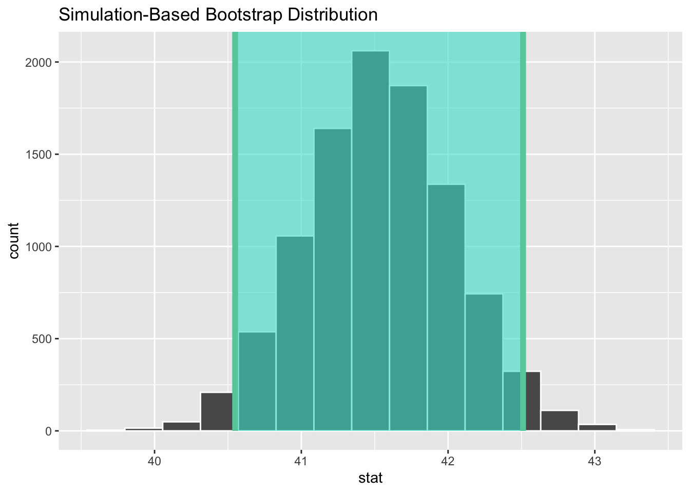
Figure 4.7: Bootstrap Distribution with Shaded Confidence Interval
Above, the CI endpoints that had previously been computed using the percentile method are sent to the shade_ci() function as a vector. However, it is perhaps more convenient to store the output from get_ci() into a variable as shown below, and then send the stored CI to the shade_ci() function. The code below produces the exact same plot shown in Figure 4.7, which shades the bootstrap distribution between its 2.5th and 97.5th percentiles.
# Store the get_ci() results into a variable
percentile_ci <- bootstrap_distribution %>%
  get_ci(level=.95, type = "percentile")
# Send the stored get_ci() results to shade_ci()
bootstrap_distribution %>%
  visualize() +
  shade_ci(endpoints = percentile_ci)      # percentile_ci contains the CI endpoints
Before moving on to further demonstrate the Infer package, a couple comments are in order. First, the get_ci() and shade_ci() functions also have longer names, get_confidence_interval() and shade_confidence_interval(). Those longer-named functions work exactly the same, so we prefer using the shorter names. Second, all of the above could be accomplished without Infer, simply by using dplyr and ggplot2. Infer provides handy functions for Cls (and hypothesis tests), often using dplyr and ggplot2 functions behind the scenes, but in general Infer is no match for the versatility of dplyr and ggplot2 for data wrangling and plotting.
Again for the sake of comparison, we’ll return to the tvhours_2018 data for which a theory-based single-proportion CI was constructed in Section 4.2. Then Section 4.7 computed bootstrap simulation-based Cls for comparison. Recall the calculation (using dplyr) for the proportion of couch potatoes in the tvhours_2018 data as shown below. For each row in the table, the Boolean logical expression tvhours >= 3 is either true (1) or false (0) which results in a 1 being added to the sum for each couch potato.
# The proportion p_hat of couch potatoes - computed using dplyr
tvhours_2018 %>%
  summarize( num_couch_potatoes = sum(tvhours >= 3),  n = n(),  p_hat = num_couch_potatoes/n )
The main hurdle to overcome to use the Infer package to do the same calculation is how the specify() function works for single-proportion bootstrap calculations. For such a calculation, the specified response variable must be a categorical variable with EXACTLY two distinct values. For example, suppose there is a categorical variable named turtle_speed whose only values are slow and fast. Then the function call to specify the response variable to bootstrap the proportion of fast turtles (most likely a small proportion) would be as follows:
specify(response = turtle_speed, success = "fast")
The value of the success parameter must be a character string. The Infer specify() function is not flexible enough to accept a Boolean expression to define success based on the comparison of a numeric variable like \(tvhours >= 3\). Thus, the following does NOT work to identify couch potatoes.
# Can't use logical expression to define success
specify(response = tvhours, success = "tvhours >= 3")    # OOPS - Error
To overcome that, some data wrangling is in order. We’ll simply create a two-value categorical variable to identify couch potatoes using the dplyr mutate() function as shown below. The new is_potato variable is assigned the truth value of each tvhours >= 3 comparison.
tvhours_2018_with_potatoes <- tvhours_2018 %>%
  mutate(is_potato = (tvhours>=3))  # new column is_potato = TRUE/FALSE
tvhours_2018_with_potatoes
## # A tibble: 833 × 2
##    tvhours is_potato
##      <dbl> <lgl>
##  1       1 FALSE
##  2       1 FALSE
##  3       4 TRUE
##  4       2 FALSE
##  5       3 TRUE
##  6       3 TRUE
##  7       2 FALSE
##  8       5 TRUE
##  9       0 FALSE
## 10       1 FALSE
## # ℹ 823 more rows
Having properly wrangled the data, the Infer package can be employed to construct a single-proportion bootstrap distribution and a confidence interval. The dplyr code that produced the same single-proportion bootstrap analysis in Section 4.7 is not shown below, but it might be worth a few seconds to compare that code with the more streamlined Infer code below.
# Compute the single-proportion bootstrap distribution
bootstrap_distribution <- tvhours_2018_with_potatoes %>%
  specify(response = is_potato, success = "TRUE") %>%
  generate(reps = 10000, type = "bootstrap") %>%
  calculate(stat = "prop")

# Compute the SE method bootstrap CI
se_ci <- bootstrap_distribution %>%
  get_ci(level=.99, type = "se", point_estimate=.340)
se_ci
## # A tibble: 1 × 2
##   lower_ci upper_ci
##      <dbl>    <dbl>
## 1    0.298    0.382

# Visualize the results
bootstrap_distribution %>%
  visualize() +
shade_ci(endpoints = se_ci) 
The results are the same as the simulation-based bootstrap SE CI constructed in Section 4.7 using dplyr. Observe above that the point estimate sent to the get_ci() function is the sample stat \(\hat{p}\) we had previously computed in Section 4.7. As shown below, a quick calculation using Infer functions spits out the same value if the bootstrap generate() part is left out.
# Calculate original sample proportion (by leaving out call to generate() bootstrap samples)
tvhours_2018_with_potatoes %>%
  specify(response = is_potato, success = "TRUE") %>%
  calculate(stat = "prop")
## Response: is_potato (factor)
## # A tibble: 1 × 1
##    stat
##   <dbl>
## 1 0.340
Some extra data wrangling may be required to use Infer, but that does not diminish its overall merits. For the two Infer bootstrap examples above, the corresponding dplyr code is somewhat less streamlined, but still not too much more complicated. However in the next example below, and especially in the next chapter when the Infer package is used for simulation-based hypothesis testing, the amount of technical programming complexity that Infer performs for you behind the scenes is well worth the trade-off of some pre-analysis data wrangling required to put the sample data into a format usable by Infer. That’s often true with programming tools in general, especially well-conceived ones that become popular. The long term benefit of the tool significantly outweighs the the start-up cost incurred in learning how to use it.
For the final example of this section, we once again return to some familiar data so that the main focus of the example is learning to use the Infer package. Section 4.4 used the gss_survey data to construct a theory-based difference of proportions CI to compare the proportion of married survey respondents that are couch potatoes to the proportion of non-married ones.
The call to do such a calculation using Infer will be calculate(stat = "diff in props" .... However, for a “diff of” CI the specify() function call that identifies the variables to be used must also include an explanatory variable as shown below.
specify(response = is_potato, success = "TRUE" , explanatory = married_status)
In other words, can the difference in marital status explain whether or not a person is a couch potato?
The catch here is that with Infer, an explanatory variable like married_status must be a categorical variable with EXACTLY two values, perhaps “married” and “single” in this case. Infer uses those two distinct categories to divide the data into two distinct subsets for the “difference of” analysis.
But the status column in the gss_survey data contains several categories: “Married”, “Never married”, “Divorced”, “Single”, etc. That was easily overcome in the theory-based approach in Section 4.4 since each proportion was computed separately by doing filter(status == "Married") in one calculation and then filter(status != "Married") in another to grab all the records in the table with NOT married status.
For Infer, the data needs to be transformed by adding a new married_status categorical column with exactly two values as shown below. The first part of the wrangle is the same as in previous examples. The new part is the case_when() part that creates a new two-category married_status column. Based upon the Boolean status comparisons, the new column is either assigned the string “married” or “single”, effectively directing all (status != "Married") survey records into the “single” category. The is_potato column could also be mutated into existence using case_when(), but that one is easier to just wrangle straight into truth values.
gss_survey_2018_wrangled <- gss_survey %>%
  filter(year == "2018") %>%
  drop_na(tvhours,status) %>%
  mutate(is_potato = (tvhours>=3)) %>%
  mutate(married_status = case_when(
                              (status == "Married") ~ "married",
                              (status != "Married") ~ "single",
                          )
  ) %>%
  select(tvhours,is_potato,status,married_status)
gss_survey_2018_wrangled
## # A tibble: 833 × 4
##    tvhours is_potato status        married_status
##      <dbl> <lgl>     <chr>         <chr>
##  1       1 FALSE     Married       married
##  2       1 FALSE     Married       married
##  3       4 TRUE      Widowed       single
##  4       2 FALSE     Married       married
##  5       3 TRUE      Divorced      single
##  6       3 TRUE      Separated     single
##  7       2 FALSE     Never married single
##  8       5 TRUE      Widowed       single
##  9       0 FALSE     Never married single
## 10       1 FALSE     Married       married
## # ℹ 823 more rows
Now that the data is properly formatted, the “diff in props” bootstrap is easily computed as shown below. Notice the order parameter in the calculation, whose value is a vector with the order for the “difference of” comparison: either \((\hat{p}_{single} - \hat{p}_{married})\) or \((\hat{p}_{married} - \hat{p}_{single})\). We chose
to list “single” first since that is the larger of the two proportions being compared, ensuring that at least the right endpoint of the resulting CI will be positive. But either order works just fine.
bootstrap_distribution <- gss_survey_2018_wrangled %>%
  specify(response = is_potato, success = "TRUE", explanatory = married_status) %>%
  generate(reps = 10000, type = "bootstrap") %>%
  calculate(stat = "diff in props", order = c("single","married"))

bootstrap_distribution %>%
  get_ci(level=.95, type = "percentile")
## # A tibble: 1 × 2
##   lower_ci upper_ci
##      <dbl>    <dbl>
## 1   0.0297    0.156

bootstrap_distribution %>%
  get_ci(level=.95, type = "se", point_estimate=(.383-.291))
## # A tibble: 1 × 2
##   lower_ci upper_ci
##      <dbl>    <dbl>
## 1   0.0281    0.156
For comparison, both bootstrap CI methods were computed above. The “difference of” point_estimate had been calculated in Section 4.4. Also in that section, the theory-based CI was calculated to be \([.0281, .1559]\) which differs from the above Cls somewhat. The tvhours data easily satisfies the assumptions required for trusting the theory-based CI. But the theory-based approach is itself based upon two approximations (normal for binomial, and also \(\hat{p}\) for \(p\)).
Recalling the previous discussions, choosing to trust the theory-based vs simulation-based analysis could simply come down to what a scholarly journal or regulatory agency might prefer. They all agree to about two decimal places, so it’s quite possible that level of accuracy is sufficient. The tvhours data is significantly skewed as can be seen in the histogram shown in Section 4.2, so if the situation calls for a simulation-based CI, then the percentile method would probably be the best choice.
We’ll conclude this section with some final subtleties about the Infer package. Calls to the specify() function can be simplified by using the optional formula parameter. For example, the following two function calls are equivalent.
# Equivalent function calls
specify(formula = is_potato ~ married_status, success = "TRUE")
specify(response = is_potato, success = "TRUE", explanatory = married_status)
Perhaps “simplified” wasn’t the best choice of words above. The formula version is more concise, but perhaps harder to understand. Such a formula is of the general form formula = response_var ~ explanatory_var, thereby eliminating individual response and explanatory parameters. If there is no explanatory variable in the analysis, the formula version must be given as formula = response_var ~ NULL. For relatively simple cases like above either type of notation suffices. But for more complex analyses, the formula parameter provides more flexibility.
Since the above example was using Infer for “difference of means”, we’ll conclude this section with a quick note about “difference of means” bootstraps using Infer. The code below assumes that var1 contains numerical data suitable for calculating means, and the explanatory categorical variable var2 has exactly two distinct values “categoryA” and “categoryB” or whatever. With those assumptions, the code below should be self explanatory having discussed the previous example in detail. Note that no success value is specified in an analysis about a mean rather than a proportion.
4.10 Resources
The R scripts provided below contain code from the main examples featured in this chapter. The scripts are numbered to keep them organized in roughly the same order that the examples were presented. The script numbers do not correspond to section numbers within this chapter.
Download a Zip archive containing all the scripts listed below:
Click on Script for Source Code:
