Chapter 5 Hypothesis Tests and Simulations
The following packages are required for this chapter.
This chapter first provides an overview Hypothesis Tests using traditional theory-based methods to explore the terminology and concepts. The underlying mathematics are highlighted, but not rigorously explored. R’s built in functions for conducting theory-based tests are introduced. Most of this chapter is then focused on simulation-based hypothesis tests, using Bootstrap and other interesting computational techniques such as random draw sampling and permutation re-sampling. The Infer package is used to facilitate the simulation-based Hypothesis Tests. Finally, after the various hypothesis testing examples presented in this chapter, it circles back and discusses some subtleties related to hypothesis tests to provide additional insight into the topic.
5.1 Theory and Concepts
With the rise of craft soft drinks (or perhaps craft beers) being marketed by small companies, a consumer advocacy group wants to test whether the bottles being sold actually contain 12oz of soda as advertised. That is, they wish to test whether the unknown population mean is actually \(\mu=12\). This is formulated as a Hypothesis Test as follows:
| Null Hypothesis \(H_0\): | \(\mu = 12\) | average bottle contains 12oz of soda |
| Alternative Hypothesis \(H_A\): | \(\mu \neq 12\) | average is different from 12oz |
| Confidence Level: 95% \((\alpha = .05)\) |
Hypothesis tests are resolved by assuming that the Null Hypothesis \(H_0\) is TRUE. In order to reject \(H_0\), there needs to be very strong evidence that the Alternative Hypothesis \(H_A\) should be accepted instead. For example for the above test, if a random sample is taken and the sample mean \(\bar{x}\) is “very close” to 12, then that would NOT be sufficient evidence to reject \(H_0\) even though \(\bar{x}\) is slightly different from 12. But if \(\bar{x}\) is “significantly different” from 12, then there would be sufficient evidence based upon the sample to reject \(H_0\) in favor of \(H_A\). In more colloquial language, \(H_0\) is assumed to be the status quo (how things are, the true state of the universe), and that is only rejected through strong evidence about which you are quite confident, perhaps at 95% level as in the above test. It’s not appropriate to reject the status quo (what is assumed to be the true state of the universe) based upon minimal (scant, flimsy, weak, …) evidence.
Of course, the notions of “very close” and “significantly different” used above need to be quantified using probability theory. To test the above hypothesis about a mean, a random sample of size \(n\) bottles will be selected and measured. Of course, proper sampling methodology will be used to ensure the sample is sufficiently random.
Recall from the discussion in Section 4.3 that the following statistic computed from the sample mean \(\bar{x}\) and standard deviation \(s\) is modeled by a T distribution with \(n-1\) degrees of freedom.
\[t = \frac{\bar{x} - \mu}{\frac{s}{\sqrt{n}}}\]
In the context of hypothesis tests, the computed value of \(t\) above is called a test statistic. It quantifies sampling variation probabilities by comparing the observed \(\bar{x}\) to the hypothesized \(\mu = 12\). The magnitude of the difference \((\bar{x} - \mu)\) is “measured” by dividing by the estimated sampling error \(SE=\frac{s}{\sqrt{n}}\). It follows that a \(T_{n-1}\) distribution gives the probability of how likely the computed test statistic \(t\) is to occur in a random size \(n\) sampling process. For a hypothesis test with a 95% confidence level, the situation is depicted in Figure 5.1.
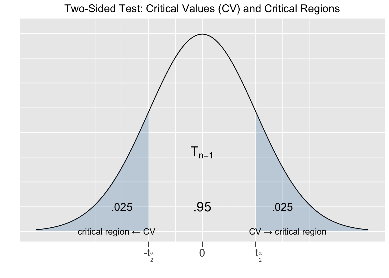
Figure 5.1: Two-Sided Hypothesis Test
The value of \(t_{frac{\alpha}{2}}\) is computed from a \(T_{n-1}\) distribution exactly like it is done for confidence intervals. In this context, each value \(\pm t_{\frac{\alpha}{2}}\) is called a Critical Value (CV) for the hypothesis test. This is a Two-Sided test since the alternative hypothesis \(H_A\) involves \(\neq\), which indicates a two-sided alternative. That is, the alternative can be either larger or smaller than the null hypothesis \(H_0\) assumption.
Each critical value defines a Critical Region of the test. If the computed value of the test statistic \(t\) falls within a critical region, \((-\infty , -t_{\frac{\alpha}{2}}]\) or \([t_{\frac{\alpha}{2}}, \infty)\), then the null hypothesis is rejected in favor of the alternative hypothesis, since that means that the difference \((\bar{x} - \mu)\) was significant. Otherwise, if the computed value of the test statistic \(t\) falls outside of a critical region, then the conclusion is that the sample does not provide sufficient evidence to reject \(H_0\).
That is consistent with the notion that rejecting \(H_0\) (the status quo) should require very “strong” evidence. The \(T_{n-1}\) distribution shown in Figure 5.1 gives probabilities for the test statistic \(t\) (which measures the difference \(\bar{x} - \mu\)) for all possible size \(n\) samples. If the test statistic \(t\) computed for the hypothesis test falls in a critical region (outside the middle 95%), then the sample mean was very unusual (5% or less probability of occurring) compared to the null hypothesis assumption for the population mean. That’s certainly sufficient evidence based on the sample for NOT trusting the null hypothesis. Conversely, if the test statistic \(t\) falls in the middle 95% region, then the sample supports \(H_0\) since it’s typical of what’s expected of size \(n\) samples if the \(H_0\) assumption is true. If the test statistic \(t\) aligns perfectly with the \(H_0\) assumption for \(\mu\), giving \((\bar{x} - \mu)=0\), then the test statistic falls exactly in the middle of the T distribution.
To put these ideas to the test (literally and figuratively), suppose the consumer advocacy group first wants to apply the 95% hypothesis test outlined above to the Largess Soda Company. To that end, the following random sample of size \(n=50\) of bottles of their soda is collected (hopefully containing at least one bottle of root beer). You should be quite familiar with the R code that imports a CSV data file, generates a histogram, and calculates summarize() statistics, so we have not shown it here.
##   ounces
## 1   11.9
## 2   12.1
## 3   12.2
## 4   11.9
## 5   12.0
## 6   12.1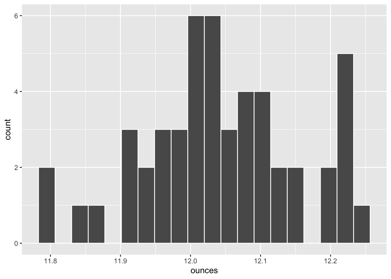
##   sample_mean sample_sd
## 1     12.0422    0.1122
The critical values computation for the two-sided test is the same as with a 95% confidence interval, sending the “quantile t” function the area under the curve to compute the positive \(t_{\frac{\alpha}{2}}\) value.
# Critical Value for 95% Two-Sided Test
t_alpha2 <- qt(.975, df=49)  # .975 = 1 -.025
t_alpha2
## [1] 2.00958
This means the critical regions (reject null hypothesis) for the computed test statistic \(t\) are \(t\le -2.00958\) and \(t\ge 2.00958\). Using the above sample statistics, computing the test statistic \(t\) is easily accomplished.
# Test Statistic based upon above sample.
t_test_stat <- (12.0422 - 12)/(.1122/sqrt(50))
t_test_stat
## [1] 2.65953
Since \(t=2.66\) falls into a critical region, the conclusion is that the sample supports rejecting the null hypothesis \(H_0\) in favor of the alternative \(H_A\). That is, based upon the sample, it is reasonable to conclude with 95% confidence that their bottles of soda do NOT contain 12oz of soda on average. Since the sample mean \(\bar{x}=12.042\) is actually greater than 12, it seems that the Largess Soda Company is living up to its name.
Instead of reporting how a computed test statistic compares to the critical values - whether it falls in a critical region or not - the results of a hypothesis test are usually reported by computing a p-value.
p-value for Hypothesis Test
Given an observed sample of size \(n\), the p-value (probability value) is the probability that ANY other sample of size \(n\) would result in a test statistic at least as “extreme” (further away from 0) as the test statistic computed from the observed sample.
A test statistic value further away from 0 means that \((\bar{x} - \mu)\) would be larger, meaning the the sample mean \(\bar{x}\) is further away from the null hypothesized value of \(\mu\), meaning the sample is more extreme relative to the null hypothesis.
For a two-sided test, being extreme relative to the null hypothesis goes in both directions, hence the p-value is the area under both tails as shown as the red-shaded areas in Figure 5.2.
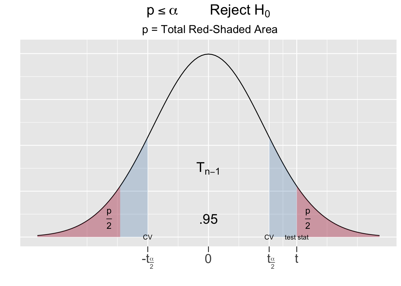
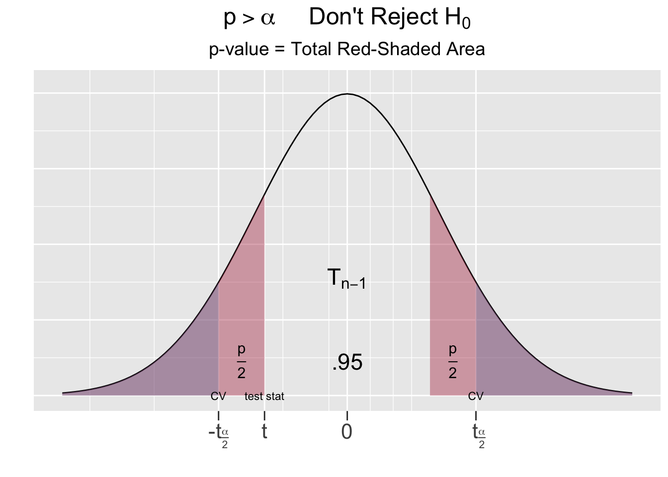
Figure 5.2: The P-Value for Two-Sided Hypothesis Test
The left side of Figure 5.2 shows the outcome of the test on the Largess Soda Company’s bottling practices, where the test statistic \(t=2.65\) fell inside the critical region. The total combined red shaded tail areas left side of Figure 5.2 are computed below using the pt() (probability t) function. It was easiest to compute the left \(\frac{p}{2}\) tail area using \(-t\), the negative of the test statistic, and then multiplying it by 2. However the same result can be obtained using \(t\) or both \(\pm t\) as shown in the comments below.
p_value <- 2 * pt(-2.66, df=49)   # 2 * single tail area p/2
p_value
## [1] 0.0105309
# same as 2 * (1 - pt(2.66, df=49))
# same as pt(-2.66, df=49) + (1 - pt(2.66, df=49))
Using probability notation, the p-value computed above is the sum of both red-shaded tail areas \(p = P(t<-2.66) + P(t>2.66) = .011\). Recall that the blue-shaded area on the left side of Figure 5.2 is \(\alpha=.05\) for a 95% test. Thus, the p-value is less than \(\alpha\).
The other possible outcome of a hypothesis test is depicted on right side of Figure 5.2, where the test statistic falls outside the critical region. In that case, the combined red-shaded tail area would be greater than the blue-shaded area \(\alpha\) (which looks purple being underneath the red). This suggests the following principle:
\(p\le\alpha\) if and only if the test static falls into a critical region
To resolve a hypothesis test, compare the p-value computed from the sample to \(\alpha\). If \(p\le\alpha\), the null hypothesis \(H_0\) is rejected in favor of the alternative. If \(p\gt\alpha\), there is not sufficient evidence to reject \(H_0\).
In a two-sided test, if the test statistic had been of the same magnitude but instead negative \((t = -2.66)\), the p-value would be exactly the same. Notice in Figure 5.2 that \(\pm t\) for the test statistic results in the exact same red-shaded area.
The p-value method for resolving a hypothesis test is EXACTLY equivalent to the critical region method. In practice, either method is an acceptable way to report the result of a hypothesis test. But in general, reporting the p-value is preferred since comparing \(p\) to \(\alpha\) is more concise and meaningful since \(p\) and \(\alpha\) are both probabilities which impart an intuitive meaning. In the Largess Soda Company bottling test, the probability that ANY sample is “more extreme” relative to \(H_0\) than the observed sample is \(p=.011\), which intuitively compares to the \(\alpha=.05\) probability tolerance defined by the hypothesis test. In contrast, reporting the value of the test statistic \(t=2.66\) and the critical critical region boundaries \(\pm2.0096\) results in a handful of x-axis numbers that don’t have intuitive meaning.
Fortunately, the core R t.test() function makes it easy to resolve a theory-based hypothesis test without having to do all of the calculations manually. For example, the Largess Soda Company bottling test can be resolved with only one t.test() function call as shown below. The soda_largess table loaded from a CSV file below contains the exact same soda ounces sample data that was used above.
soda_largess <- read_csv("http://www.cknuckles.com/statsprogramming/data/soda_sample_largess.csv")
t.test(soda_largess$ounces, alternative = "two.sided", mu = 12 , conf.level = 0.95)
##
##  One Sample t-test
##
## data:  soda_largess$ounces
## t = 2.66, df = 49, p-value = 0.0105
## alternative hypothesis: true mean is not equal to 12
## 95 percent confidence interval:
##  12.0103 12.0741
## sample estimates:
## mean of x
##   12.0422
Notice that the output of the t.test() function contains most of the information that was calculated manually further above. In particular, the p-value \(p = 0.0105\) immediately indicates to reject the null hypothesis in a 95% \((\alpha=.05)\) test in favor of the alternative. Other information includes the sample mean \(\bar{x}\) and the computed test statistic \(t\). Notice that it doesn’t even report the critical values \(\pm t_{\frac{\alpha}{2}}\) since they are not needed to resolve the test using the p-value.
The output also reports the theory-based confidence interval centered around the sample mean \(\bar{x}\). Recall that the endpoints of such a theory-based confidence interval would be computed as \(\bar{x} \pm t_{\alpha/2} \cdot \frac{s}{\sqrt{n}}\). In fact recalling Section 4.3, this CI formula was derived from the exact same T Statistic formula that computes the test statistic for the hypothesis test presented earlier in this section. Thus, the CI can also be used to resolve a hypothesis test.
Back to the Largess Soda Company bottling test which results in a 95% CI of \([12.01, 12.07]\) as computed by the t.test() function above. So we have 95% confidence that the true, unknown population mean \(\mu\) of ounces per bottle falls within that interval. But the CI does NOT contain the null hypothesis assumption of \(\mu=12\). Therefore, based upon the CI, it is logical to reject the null hypothesis that \(\mu = 12\) in favor of the alternative that \(\mu \neq 12\).
The above observation about the hypothesis test and CI for the Largess Soda Company bottling test generalizes to the following principle:
\(p\le\alpha\) if and only if the \(\bar{x}\)-centered CI does NOT contain the Null Hypothesis Assumption
The prefered way to report on the results of a hypothesis test is to provide the p-value. But to convey more information, most publications prefer listing both the p-value and the CI, even though the same conclusion can be drawn from either. The p-value conveys how unusual probabilistically an observed sample is compared to the Null Hypothesis Assumption. The CI provides an interval estimate for the unknown population parameter that’s independent of the Null Hypothesis Assumption.
For another example, suppose that the consumer advocacy group decides to test another soft drink manufacturer using the exact same two-sided \(H_0: \mu = 12\) hypothesis test. This time the following random sample of size \(n=50\) bottles is collected from stores selling bottles of soda from Veracious Bottling, Inc. Again, we won’t show the code that imports the CSV data file, generates the histogram, and calculates summarize() statistics since such familiar code won’t add to the current discussion.
##   ounces
## 1  11.86
## 2  11.98
## 3  12.13
## 4  11.84
## 5  11.95
## 6  11.97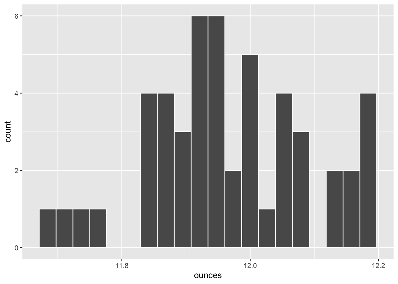
##   sample_mean sample_sd
## 1     11.9678  0.124496
In the first example in this section, it was helpful to see the test statistic formula and compare its computed value to the critical values \(\pm t_{\alpha/2}\). It was also helpful to manually compute the p-value to provide insight on exactly what a p-value is. Reflecting upon the similarity between the test statistic and CI formulas also provides valuable insight to what hypothesis tests are all about. But at this point, we’ll dispense with the manual calculations and simply send the data collected for Veracious Bottling, Inc. to the t.test() function as shown below. The T test is exactly the same as before, except that the data is different.
soda_veracious <- read_csv("http://www.cknuckles.com/statsprogramming/data/soda_sample_veracious.csv")
t.test(soda_veracious$ounces, alternative = "two.sided", mu = 12 , conf.level = 0.95)
##
##  One Sample t-test
##
## data:  soda_veracious$ounces
## t = -1.829, df = 49, p-value = 0.0735
## alternative hypothesis: true mean is not equal to 12
## 95 percent confidence interval:
##  11.9324 12.0032
## sample estimates:
## mean of x
##   11.9678
There are a few important things to note in the above T test output. Most importantly, since \(p>\alpha\) \((.074>.05)\), the test fails to reject the null hypothesis that \(\mu = 12\). Stating the conclusion is that easy when armed with the p-value! Based upon this sample, Veracious Bottling is indeed seems to be providing its customers 12oz of soda on average. In most cases it would be sufficient stop there, and also report the CI of \([11.932, 12.003]\) for informative purposes. Observe that the CI contains the null hypothesis assumption \(\mu = 12\), which equivalently indicates the test fails to reject the null hypothesis.
Even though it’s not necessary in stating the conclusion, it’s also helpful to remember what’s going on behind the scenes. The test statistic was computed to be \(t = -1.829\). That’s roughly the situation shown on the right side of Figure 5.2, where the test statistic is negative, but not in a critical region. The p-value (red-shaded area) is therefore greater than \(\alpha=.05\) (blue shaded area hiding behind the red). Again observe in Figure 5.2 that in a two-sided test, it’s the magnitude of the test statistic (not its \(\pm\) sign) that determines the red-shaded area. Hence, if the test statistic for the Veracious Bottling test had been instead been \(t = 1.829\) (just switched to positive), the p-value would be exactly the same.
In yet another test using the exact same two-sided \(\mu = 12\) hypothesis test, a random sample is taken of \(n=50\) bottles of soda made by Curmudgeon Beverage, LLC. This time we’ll skip showing the data, histogram, and sample stats and get straight to the point: import the data and run the T-test. Like the other soda data used above, the soda_curmudgeon data appears to be normal-ish when plotted via histogram, and you can see the sample mean \(\bar{x} = 11.91\)oz at the bottom of the t.test() output below.
soda_curmudgeon <- read_csv("http://www.cknuckles.com/statsprogramming/data/soda_sample_curmudgeon.csv")
t.test(soda_curmudgeon$ounces, alternative = "two.sided", mu = 12 , conf.level = 0.95)
##
##  One Sample t-test
##
## data:  soda_curmudgeon$ounces
## t = -7.635, df = 49, p-value = 6.92e-10
## alternative hypothesis: true mean is not equal to 12
## 95 percent confidence interval:
##  11.8863 11.9337
## sample estimates:
## mean of x
##     11.91
The p-value above is \(p=.000000000692\) after converting from scientific notation. That’s effectively 0, which means that the 95% test rejects the null hypothesis of \(\mu = 12\). From the sample it appears that the Curmudgeons, whether intentionally or not, are cheating their customers with \(\bar{x} = 11.91\)oz bottles of soda on average.
One thing to note in this example is the extremely small p-value. It is fairly common in various statistical software (not just R) to report such a p-value as simply 0 because that’s what it rounds off to after several decimal places. That can be confusing because a p-value can technically NEVER be 0 since the tails of a T distribution (or normal one) approach 0 asymptotically, never reaching 0. There is always some tail area, no matter how small.
Similarly, suppose that a p-value in a two-sided test is close to 1, or perhaps even equal to 1. For example, suppose one of the soda samples above had mean \(\bar{x} = 12\), exactly matching the null hypothesis \(\mu = 12\). In that case the test statistic would be precisely 0, in the exact middle of the T distribution. The p-value would then be 1 since both tail areas would start at 0, totaling all the area under the entire distribution. Similarly, a sample mean \(\bar{x}\) near 12 would give a p-value near 1. Obviously in all such cases, the sample would strongly support the null hypothesis.
We now turn to the concept of a One-Sided Hypothesis Test. For the sake of comparison, we’ll stick with the consumer advocacy group that’s testing bottling practices of soft drink manufacturers. The hypothesis test outlined below is Left-Sided since the alternative hypothesis is \(\mu \lt 12\).
| Null Hypothesis \(H_0\): | \(\mu = 12\) | average bottle contains 12oz of soda |
| Alternative Hypothesis \(H_A\): | \(\mu \lt 12\) | average is less than 12oz |
| Confidence Level: 95% \((\alpha = .05)\) |
Otherwise the hypothesis test is EXACTLY the same. A Right Sided test would have \(\mu \gt 12\) as the alternative hypothesis. A left-sided example will be sufficient to show the nature of One-Sided tests in general, since the concepts are the same for right-sided tests. Figure 5.3 provides a visualization of a Left-Sided test.
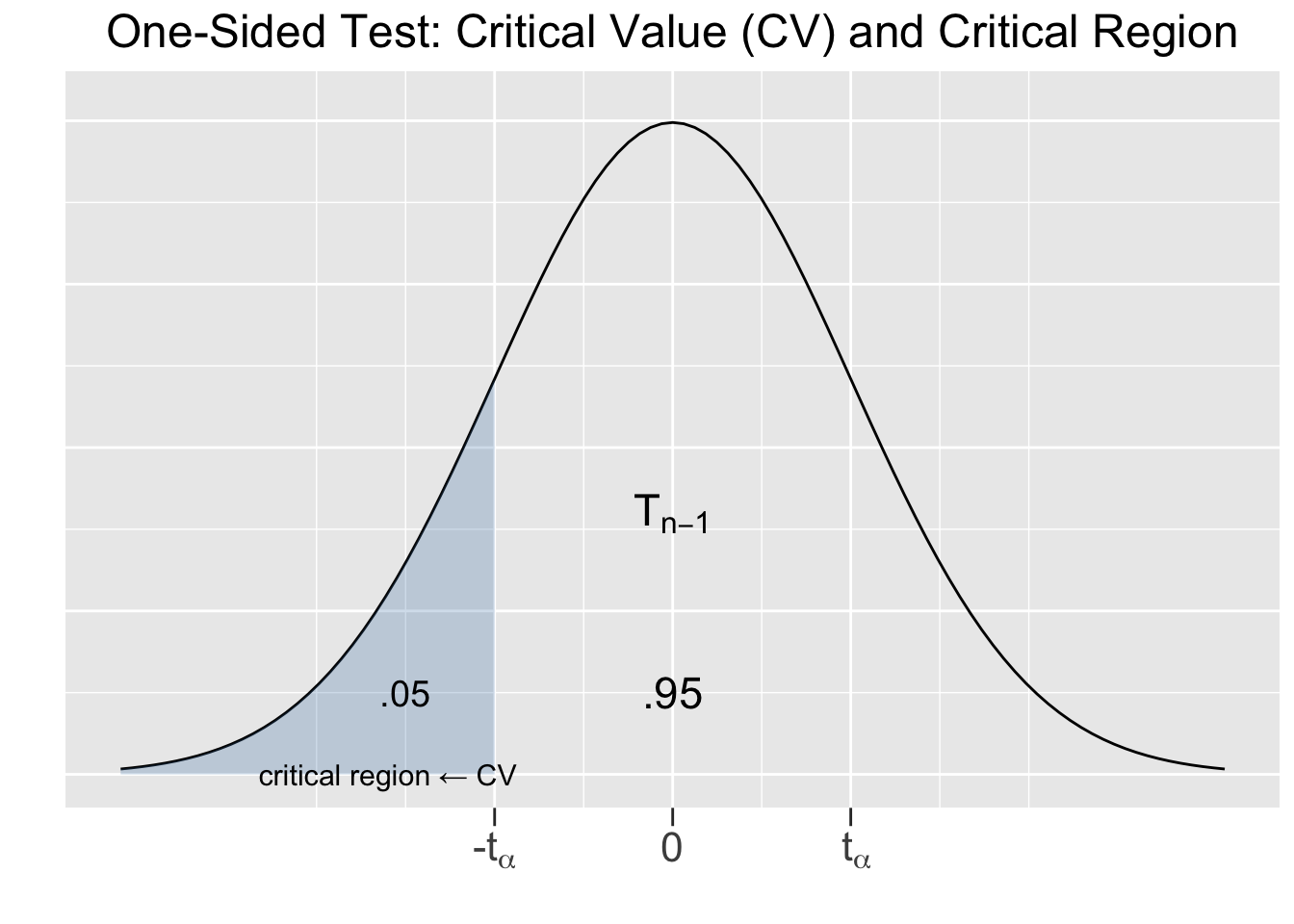
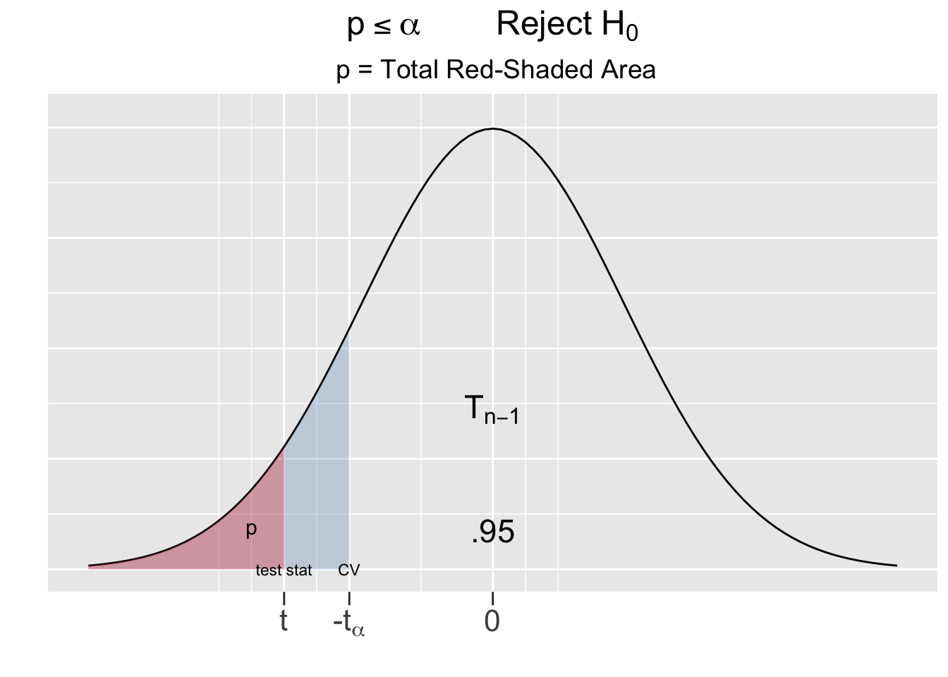
Figure 5.3: One-Sided Hypothesis Test
On the left side of Figure 5.3, the obvious difference is that the critical region and critical values only go in the direction of the alternative hypothesis, \(\lt\) in this case. The only critical value for the left-sided test is \(-t_{\alpha}\). Since there is only one tail in play with area \(\alpha=.05\), the critical region is defined by \(t_{\alpha}\) (instead of \(\frac{\alpha}{2}\)). The conclusion of the hypothesis test is as expected: if the test statistic computed from the sample falls into the critical region, then the null hypothesis is rejected in favor of the alternative hypothesis.
The right side of Figure 5.3 shows that the p-value in a one-sided test is a single tail area. Remember, the p-value is the probability that ANY other sample of size \(n\) results in a test statistic that is at least as “extreme” as the test statistic computed from the observed sample. For a one-sided test, being extreme goes only in the direction of the alternative hypothesis \(H_A\) that’s competing with \(H_0\). Other than that, the p-value for a one-sided is interpreted in the same way: if \(p\le\alpha\) then the null hypothesis is rejected in favor of the alternative hypothesis. Otherwise if \(p>\alpha\), the sample doesn’t provide sufficient evidence to discredit the null hypothesis.
To contrast with the two-sided hypothesis conducted further above on the Veracious Bottling sample, suppose the consumer advocacy group instead runs the left-sided test as defined above on the same sample data. The only difference in the t.test() function call below is that the value of the alternative parameter is given as “less” (instead of “two.sided”). The value for a right-sided test would be “greater”.
soda_veracious <- read_csv("http://www.cknuckles.com/statsprogramming/data/soda_sample_veracious.csv")
t.test(soda_veracious$ounces, alternative = "less", mu = 12 , conf.level = 0.95)
##
##  One Sample t-test
##
## data:  soda_veracious$ounces
## t = -1.829, df = 49, p-value = 0.0368
## alternative hypothesis: true mean is less than 12
## 95 percent confidence interval:
##     -Inf 11.9973
## sample estimates:
## mean of x
##   11.9678
The most obvious things to note about the results of the one-sided T test are the p-value and the reported 95% CI. Since \(.0368\lt.05\), the conclusion from the p-value is to reject the null hypothesis in favor of the alternative that \(\mu \lt 12\). The one-sided test results in a one-sided confidence interval \((-\infty,11.997)\) that stretches to infinity in the direction of the test. The CI results in the same conclusion since the value of 12 hypothesized by \(H_0\) is not in the CI.
t.test()DirectionThe
alternativevalue set in thet.test()function should match the “direction” of the alternative hypothesis:
alternative="two.sided",alternative="less", oralternative="greater"
One takeaway from this example is the notion of one-sided confidence intervals. That topic is often introduced in stats textbooks at the same time as two-sided confidence intervals. We have saved it for now because the concept is more natural in the context of one-sided hypothesis tests, where the hypothesized alternative only goes in one direction. Mathematically, this left-sided CI would be given by \((-\infty,\bar{x}+t_{\alpha}\cdot SE)\). The main difference from a standard two-sided CI (other than the \(-\infty\)) is that the SE multiplier is \(t_{\alpha}\) (instead of \(\frac{\alpha}{2}\)). The number \(t_{\alpha}\) for a 95% test is the 95th percentile (tail area .05) of the T distribution, whereas \(t_\frac{\alpha}{2}\) is the 97.5th (tail area .025).
The factor of 2 difference in tail areas noted just above directly also applies to p-values. The two-sided test of the Veracious Bottling sample further above produced a p-value of \(p=0.0735\). But the one-sided test produced a p-value of \(p=0.0368\), which is precisely half. Yet the test statistic computed from the sample is EXACTLY the same in each test. In a one-sided test, the p-value is the tail area in one direction from the test statistic. In a two-sided test, that “one direction” tail area must be doubled to account for the hypothesized alternative going in both directions.
This highlights a puzzling conundrum. The above examples used the same sample of \(n=50\) bottles made by Veracious Bottling. The one-sided test (\(p=0.0368\)) calls for rejecting the null hypothesis in favor of the alternative. But the two-sided test (\(p=0.0735\)) reaches the opposite conclusion. Yet both tests were conducted at a 95% confidence level. Of course, the different outcomes are explained by the “factor of 2” differences in tail areas discussed just above. Indeed, the left tail area depicted in Figure 5.3 is twice those shown for the two-sided test in Figure 5.2.
Having presented the technical terms and concepts for hypothesis tests, it’s important to take a step back and consider the topic from a research methodology standpoint. Proper research methodology is usually a sequence of events as follows: researchers form a conjecture, a hypothesis test is designed to test the conjecture, and finally a random sample is taken from which to resolve the hypothesis test.
In fact, it’s often the case in practice - pharmaceutical research for example - that a statistical plan has to be pre-approved before the study is actually undertaken. The pre-approval usually requires a sampling plan to ensure a proper random sampling process will be used, an analysis plan to ensure proper statistical methodology is applied, and a pre-designed hypothesis test to match error tolerance with the type of study. The sample is taken (or perhaps analyzed) only after the statistical plan is set in stone.
The importance of the following principle can’t be overstated.
A Hypothesis Test is Formulated BEFORE the Sample is Taken
It it not sound statistical practice to change either the confidence level of the test OR the direction (one-sided vs two-sided) of the test after having analyzed, or perhaps even having observed, the sample data. It is not ethical for a researcher to analyze the data, then manipulate a hypothesis test to produce a pre-desired conclusion. Changing the confidence level can change the conclusion of a hypothesis test. Changing the direction of a hypothesis test can also change the conclusion.
For example, suppose the consumer advocacy group has some bias against Veracious Bottling and are hoping to prove that they are cheating customers. Bottling variation tends to go in both directions, so a two-sided test is the logical choice, perhaps even the industry standard. The above two-sided test failed to support the alternative that \(\mu \neq 12\). It would NOT be appropriate (not even legal in some situations) to notice that the sample mean is \(\bar{x}=11.966\), which is less than 12, and then to switch to a left-sided test, which is twice as likely to support the alternative hypothesis \(\mu \lt 12\) than a two-sided test at the SAME confidence level.
It would also NOT be appropriate to raise the confidence level after the sample is taken to get a smaller \(\alpha\), hence less likely that \(p\le\alpha\), to change the test result. A thorough discussion about the factors that influence the choices for the confidence level and direction of a hypothesis test is beyond the objectives of this section. That discussion is saved for Section 5.6.
The remainder of this section provides a broad overview of theory-based hypothesis tests. The same terms and concepts that were explored above for single-sample means tests also apply to single-sample proportion and two-sample “difference of” hypothesis tests. The main difference is the particular test statistic used to resolve the test. Table 5.1 summarizes common theory-based hypothesis tests.
| Hypothesis Test | Null Hypothesis | Test Statistic | Distribution of the Test Statistic |
|---|---|---|---|
| Proportion | \(p=p_0\) | \(z = \frac{\hat{p} - p_0}{\sqrt{\frac{\hat{p}(1-\hat{p})}{n}}}\) | \(N(0,1)\) |
| Mean | \(\mu=\mu_0\) | \(t = \frac{\bar{x} - \mu_0}{\frac{s}{\sqrt{n}}}\) | \(T_{n-1}\) |
| Diff Proportions | \(p_1-p_2=\delta\) | \(z =\frac{(\widehat{p_1} - \widehat{p_2})-\delta}{\sqrt{\frac{\widehat{p_1}(1-\widehat{p_1})}{n_1} + \frac{\widehat{p_2}(1-\widehat{p_2})}{n_2}}}\) | \(N(0,1)\) |
| Diff Means | \(\mu_1-\mu_2=\delta\) | \(t = \frac{(\overline{x_1} - \overline{x_2})-\delta}{\sqrt{\frac{(n_1-1)s_1^2 + (n_2-1)s_2^2}{n_1+n_2-2}} \cdot \sqrt{\frac{1}{n_1}+\frac{1}{n_2}}}\) | \(T_{n_1+n_2-2}\) |
Yikes! The test statistic formulas are a bit scary. But don’t let those details get in the way of the big picture take-aways:
- Any of the hypothesis tests in Table 5.1 could be resolved in the following EQUIVALENT ways:
- comparing the p-value computed from the test statistic to \(\alpha\)
- comparing whether the \(\bar{x}\)-centered CI contains the null hypothesis assumption
- comparing the test statistic to the critical value(s)
- The only differences are the test static formulas (obviously) and the underlying Distribution of the Test Statistic.
- The concepts regarding two-tailed vs one-tailed tests are the same.
The astute reader many have noticed the similarity between the formulas in Table 5.1 and the confidence interval formulas presented in Chapter 4. Indeed, the derivation for a CI for a single-sample mean was shown in Section 4.3. Let’s revisit that in this context. The inequality on the left below simply says that the test statistic is between the two critical values. Solving that for the null hypothesized value \(\mu_0\) results in the CI formula on the right.
\[ -z_{\alpha/2} \;\le\;\frac{\bar{x} - \mu_0}{\frac{s}{\sqrt{n}}} \;\le\; z_{\alpha/2} \;\;\;\;\;\;\;\;\;\implies\;\;\;\;\;\;\;\;\; \bar{x} - z_{\alpha/2} \frac{s}{\sqrt{n}} \;\le\; \mu_0 \;\le\; \bar{x} + z_{\alpha/2} \frac{s}{\sqrt{n}} \]
The other two-sided CI formulas presented in Chapter 4 can be similarly derived from the test statistics in Table 5.1 as summarized below.
Test Statistics and CI Formulas
The two-sided CI formulas presented in Chapter 4 are derived by solving an equation like \(-CV \le TS \le CV\) (where TS=Test Stat and CV=Critical Value) for the Null Hypothesized value (\(p_0\), \(\mu_0\), or \(\delta\)). One-sided CI’s are derived from similar one-sided inequalities. This emphasizes why hypothesis tests can be equivalently resolved using a confidence interval comparison.
We now turn to “difference of” hypothesis tests, for which the general form of the null hypothesis using \(\delta\) is shown in Table 5.1. However, the most common use of such tests is when \(\delta=0\), in which case the test simply boils down to whether \(\mu_1=\mu_2\) or \(\widehat{p_2}=\widehat{p_2}\). Thus, with \(\delta=0\) the test is to determine if differences in mean or proportion measurements from two independent populations are the same or not. Indeed, the “difference of” CI examples in Chapter 4 were all concerned with whether 0 was contained in the “difference of” CI.
The following difference of means hypothesis test is typical of a “difference of” hypothesis test.
| Null Hypothesis \(H_0\): | \(\mu_1-\mu_2=0\) | no difference in population means |
| Alternative Hypothesis \(H_A\): | \(\mu_1-\mu_2\ne0\) | population means are different |
| Confidence Level: 95% \((\alpha = .05)\) |
So that we don’t need to load any new data sets, we’ll apply the above test to two samples used in the above examples that are already imported from CSV into the following data tables in R: soda_largess (\(\bar{x}=12.0422\)) and soda_veracious (\(\bar{x}=11.9678\)). Of course, the difference of means test statistic formula could be used for manual computations, but R’s core t.test() function again makes the job easy.
# Passing in 2 data sets automatically runs a "difference" of test
t.test(soda_largess$ounces, soda_veracious$ounces,
       alternative = "two.sided", mu = 0 , conf.level = 0.95)
##
##  Welch Two Sample t-test
##
## data:  soda_largess$ounces and soda_veracious$ounces
## t = 3.139, df = 96.96, p-value = 0.00225
## alternative hypothesis: true difference in means is not equal to 0
## 95 percent confidence interval:
##  0.0273588 0.1214412
## sample estimates:
## mean of x mean of y
##   12.0422   11.9678
# The following defaults to the exact same values as above
# t.test(soda_largess$ounces, soda_veracious$ounces)
Since \(00225\lt.05\), the null hypothesis is rejected in favor of the alternative hypothesis: based upon the samples, the average amount of soda in the Largess bottles is statistically different from the average in the Veracious bottles. Equivalently, the CI reported by the test does not contain 0 thereby giving the same test result. Note also in the comments in the above code block that most of the parameters sent to the t.test() are actually the defaults when two samples are passed intot.test(). This speaks to the most common configuration for a difference of means test.
Hypothesis Terminology
The meaning of Alternative Hypothesis is intuitive. But why isn’t the Null Hypothesis given a more intuitive name, perhaps something like Primary Hypothesis? The term Null Hypothesis is actually intuitive in the context of a two-sided test where the primary hypothesis is most often a difference of 0 (null) - literally a Null hypothesis!
The reader is encouraged to run the ?t.test command in the R Studio console and see all the different options in the Help pane. In particular, the purpose of the one named var.equal was discussed in some detail in Section 4.5. The CI formula presented there, which would be derived from the big gnarly difference of means test statistic shown in Table 5.1, depends on the assumption that the two samples have approximately equal variances.
Notice that the output of the above test says “Welch Two Sample t-test” at the top. The Welch method does not require the assumption of equal variances, and is even somewhat more complicated than the difference of means formulas we have presented. The variances of the two samples used in the above difference of means example were perhaps similar enough (standard deviations were .112 and .124) to satisfy the equal variances assumption. Thus, it was probably not necessary to use the Welch test. Overriding the default by setting var.equal = TRUE in the t.test() function call causes the function to abandon the Welch method in favor of the “equal variance” method presented in this book, both for difference of means CIs and hypothesis tests. Fortunately in this case since the sample sizes are not small, running the T test either way produces almost identical results.
The purpose here is not to discuss the Welch method, which is best left to more advanced mathematical statistics books. The purpose here is to emphasize that theory-based inferential statistics is based upon assumptions that must hold in order for the underlying mathematics to be valid. Notice that we used the words “perhaps” and “probably” in the above paragraph. It’s not always obvious which is the most appropriate statistical test to use in a given situation. Indeed, even experienced statisticians sometimes debate such matters.
For another example showing that more advanced statistical tests are often used when certain assumptions don’t hold, consider R’s built in prop.test() function. Having been introduced to the t.test() function, it wouldn’t take you long to find online resources with examples of how to use prop.test() to conduct theory-based hypothesis tests about proportions. Depending upon how you use it, you may get a message that says it’s using the “Wilson score interval” or you may need to determine whether a “continuity correction” is appropriate. So again, R’s core function for implementing theory-based proportion tests might throw some unfamiliar terminology at you because of how different assumptions make certain types of theory-based tests more reliable.
Assumptions, Assumptions, Assumptions
Section 4.8 discussed in some detail the issues about all the various assumptions required for theory-based inference. Understanding the nuances of theory-based inference requires a somewhat advanced knowledge of mathematical statistics. Case in point: the above
t.test()function call defaulted to a Welch method test, which is typically covered in intermediate-level mathematical statistics textbooks. How is someone with less statistical background supposed to make sense out of all this? One answer is to learn more of the mathematical theory behind inferential statistics! Another anwser is to turn to simulation based inference, which is much less dependent on assumptions about unknown poluations. Let the sample pull itself up by it’s own bootstrap!
5.2 Simulated Tests vs Theory
The next few sections in this chapter introduce the concept of a simulation-based hypothesis test - a hypothesis test resolved using a computer simulation, rather than with mathematical theory. The previous section exclusively featured theory-based tests, both directly using test statistic formulas and also by using core R functions such as t.test() as a tool. Functions like t.test() are very handy tools that help you conduct hypothesis tests using a computer, but still use mathematical theory-based approaches behind the scenes.
This section gently introduces simulation-based hypothesis tests for a single-sample mean by comparing with the theory-based approach from the previous section. But we’ll save the details of using Infer package code for simulated tests until the next section, and instead focus on the over-arching concepts in this section.
To understand the discussion below, the reader should be familiar with the concepts of simulation-based bootstrap distributions and bootstrap confidence intervals as introduced in Sections 4.6 and @ref( bootstrap-ci), respectively.
To set a basis of comparison for concepts about simulation-based hypothesis tests, recall that theory-based hypothesis tests are typically resolved in the following ways, each of which gives the same test conclusion:
- The test statistic value is a measure of how unlikely the observed sample is assuming the null hypothesis is true. The probability that any other sample is even more unlikely - the p-value - is obtained from the underlying theory-based distribution of the test statistic. The p-value to \(\alpha\) comparison determines the outcome of the hypothesis test.
- A theory-based confidence interval, also derived from the theory-based distribution of the test statistic, is constructed around the observed sample statistic. The outcome of the hypothesis test is determined by whether the confidence interval contains null hypothesis assumption.
After summarizing above how theory-based hypothesis tests are typically resolved, we would be remiss not to re-emphasize the extent to which theory-based inference is assumption-dependent.
Simulation-Based Tests are Not Dependent on Assumptions
The “Assumptions, Assumptions, Assumptions” note at the end of the previous section emphasizes that theory-based aproaches are only reliable when certain asumptions are met. Simulation-based techniques for inferrence are more versatile since they are NOT mathematically dependent on such assumptions.
Simulation-based tests are resolved in the same ways listed above, but there is a key difference regarding the underlying distribution from which the probabilities are derived. The theory-based distribution of the test statistic is given by mathematical theory and the Central Limit Theorem. A simulation-based test also requires a probability distribution to measure how likely the observed sample is to occur assuming the null hypothesis is true. But such a distribution - a Simulation-Based Null Distribution - is constructed computationally using a simulation-based approach such as bootstrap.
Simulation-Based Null Distribution A discrete distribution constructed through a computer simulation that models sampling variation probabilities assuming that the Null Hypothesis is true. A Simulation-Based Null Distribution consists of sample statistics computed from many simulated samples, usually 10,000 or more.
For example, suppose the null hypothesis for a test for a single-sample mean is \(H_0\): \(\mu=\mu_0\). Of course, a random sample would be taken to resolve the hypothesis test. For a simulation-based test, the sample would be bootstrapped resulting in a bootstrap distribution with mean \(\bar{x}\), the same as the mean of the sample. To get a Simulation-Based Null Distribution that matches the null hypothesis \(\mu=\mu_0\), the entire bootstrap distribution is “re-centered” (shifting it left or right) so that its mean becomes \(\mu_0\). Re-centering it around \(\mu_0\) doesn’t change the shape of the distribution at all. Therefore, the resulting Null Distribution provides a Simulation-Based \(\mu_0\)-centered probability model for the sampling variation.
The next section explores the Infer package workflow that makes computing a Simulation-Based Null Distribution, and inferring from one, quite easy. For now we’ll focus only on the concept, rather than the code, by showing the results of simulation-based tests for the Largess Soda Company and Veracious Bottling, Inc examples, for which theory-based tests were conducted in the previous section. In both those examples, the null hypothesis of \(H_0\): \(\mu = 12\) was tested against a two-sided alternative at a 95% confidence level.
As computed in the previous section, the size \(n=50\) sample of bottles from the Largess Soda Company has a mean of \(\bar{x}=12.042\). The theory-based 95% test resulted in a p-value of \(p=.01\) and a 95% CI of \([12.01 , 12.07]\). From either of those results, the sample supports rejecting the null hypothesis that \(\mu = 12\) in favor of the two-sided alternative.
Figure 5.4 shows the corresponding results of a bootstrap simulation-based test, of course using the same Largess Soda Company sample data. Both the p-value and CI are the same to two decimal places as in the theory-based test, resulting in the same conclusion of rejecting the null hypothesis that \(\mu = 12\).
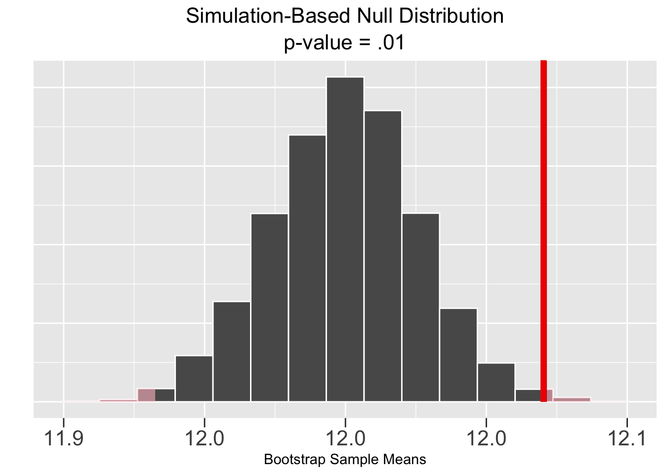
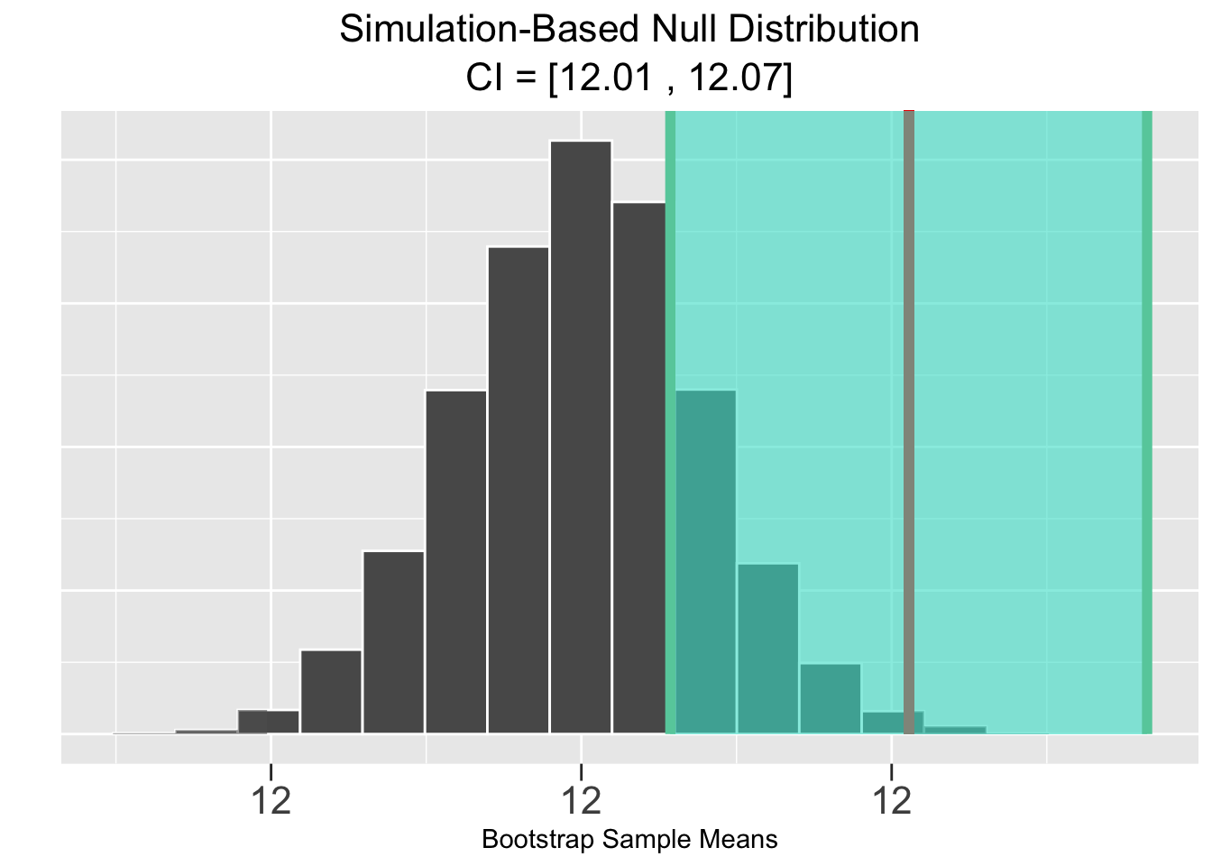
Figure 5.4: Simulation-Based Hypothesis Test: Largess Soda Company
The plots in Figure 5.4 are generated by Infer package functions. Again, more about that in the next section. The plot on the left shows the sample mean \(\bar{x}=12.042\) (vertical red line) and the p-value (pink shaded area) computed from that. Notice that half the shaded p-value area is in each tail since it’s a two-sided test. The plot on the right shows the \(\bar{x}\)-centered CI (green shaded area) which does not contain the null hypothesized value of 12.
Next, we’ll shift focus to the Veracious Bottling, Inc size \(n=50\) sample with mean \(\bar{x}= 11.97\) as computed in the previous section. The theory-based 95% test resulted in a p-value of \(p=.07\) and a 95% CI of \([11.932 , 12.003]\). From either of those results, the sample supports the null hypothesis that \(\mu = 12\), rejecting the two-sided alternative.
Figure 5.5 shows the corresponding results of a bootstrap simulation-based test, of course based upon the same sample data. Both the p-value and CI result in the same conclusion of failing to rejecting the null hypothesis that \(\mu = 12\).
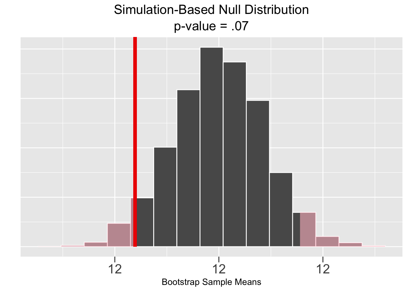
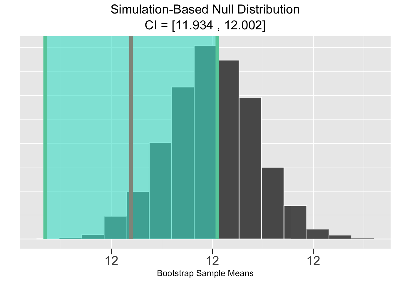
Figure 5.5: Simulation-Based Hypothesis Test: Veracious Bottling, Inc.
The Infer package plots in Figure 5.5 again show the sample mean \(\bar{x}=12.042\) and pink shaded p-value in the plot on the left, and the green shaded \(\bar{x}\)-centered CI on the right. These plots are very similar to the ones just above in Figure 5.4. But here the hypothesis test conclusion is the opposite since the p-value area is grater than \(.05\) and the CI does contain the null hypothesized value of 12.
The simulation-based p-value probabilities shaded pink in the left-most plots in the above two figures are similar in concept to p-values computed for theory-based tests as discussed at length in the previous section.
p-value for Simulation-Based Test
Given an observed sample of size \(n\), the p-value (probability value) is the probability that ANY other sample of size \(n\) would result in a sample statistic at least as “extreme” (further away from the null hypothesized value) as the sample statistic computed from the observed sample.
In Figure 5.5 just above, an \(\bar{x}\) sample statistic computed from ANY sample would be more “extreme” if it’s further away from the null hypothesized value of \(\mu=12\) than the observed sample statistic \(\bar{x}=11.97\). That notion of extreme is consistent with the pink shaded p-value area in the left plot in Figure 5.5.
Although the concept of the p-value is the same for both theory-based and simulation-based tests, there is one subtle difference. The theory-based p-value definition presented in Section 5.1 framed the notion of being extreme in terms of values of the test statistic (big formula - T or Z distribution), whereas the simulation-based p-value definition above directly refers to a sample statistic, such as a mean \(\bar{x}\).
In some cases, a theory-based test could directly use a sample statistic such as a proportion in computing a p-value. For a single-sample proportion, the CLT implies the sampling distribution of \(\hat{p}\) is approximately \(N(p_0,\left(SE\right)^2)\) where \(p_0\) is the null hypothesized value and \(SE=\sqrt{p_0(1-p_0)/n}\). The p-value for an observed sample statistic \(\hat{p}\) could be computed directly from the \(N(p_0,\left(SE\right)^2)\) distribution. Equivalently, the p-value can be computed as shown in Section 5.1 using the “normalized” test statistic \(z=(\hat{p}-p_0)/SE\) which has a standard normal \(N(0,1)\) distribution. In the normalized version, the test statistic is simply the z-score of the sample statistic.
However, the situation is somewhat different for a hypothesis test for a mean since the mathematics say the test statistic comes from a T distribution. A T distribution is somewhat similar (mean of 0 and symmetric) to a standard normal Z distribution, but a T distribution is not simply the “normalized” version of some other distribution in the same way that a Z distribution is. Therefore, the p-value for a mean \(\bar{x}\) must be obtained using the test statistic value computed from the formula and the appropriate T distribution. You can’t simply compute the p-value directly using \(\bar{x}\).
The points made by the previous paragraphs are somewhat subtle. It’s not necessary for the reader to fully comprehend those points to understand the difference between p-values for theory-based and simulation-based tests. In BOTH cases, the p-value is the probability of other samples being more extreme relative to \(H_0\) than the observed sample. For a theory-based test, the p-value is obtained using a test statistic and the distribution of the test statistic. For a simulation-based test, the p-value is obtained directly using the sample statistic and the simulation-based null distribution.
We conclude this section by noting that there are several computational techniques that are used to compute simulation-based null distributions. Above, we featured bootstrapping since that concept was already introduced in Chapter 4 and is the proper computational technique for simulation-based tests for single-sample means such as in the soda bottling examples.
The list below contains the computational techniques that will be featured for computing null distributions for various types of simulation-based hypothesis tests in the remainder of this chapter.
Computational Techniques for Simulation-Based Hypothesis Tests
- Bootstrap Sampling - Tests for single-sample means
- Random Draw Sampling - Tests for single-sample proportions
- Permutation Sampling - “Difference of” tests for both means and proportions
In the case of single-sample means as discussed in this section, a bootstrapped simulation-based null distribution is basically just a bootstrap distribution, normally centered upon the original sample mean, just re-centered upon the null hypothesis assumption. In the other cases listed above, the simulation methods so not so easily explained. Stay tuned!
5.3 Bootstrap Mean Test
Having explored the concepts in general in the previous section, this section gets straight to an example demonstrating the Infer package code to conduct a simulation-based hypothesis test for a single-sample mean. We’ll return to the Curmudgeon Beverage, LLC data that was imported from a CSV file into the soda_curmudgeon table in Section 5.1. For the sake of comparison, we’ll run the same 95% two-sided hypothesis test on the data:
| Null Hypothesis \(H_0\): | \(\mu = 12\) | average bottle contains 12oz of soda |
| Alternative Hypothesis \(H_A\): | \(\mu \neq 12\) | average is different from 12oz |
| Confidence Level: 95% \((\alpha = .05)\) |
With one exception, the code below is exactly like the Infer package code introduced in Section 4.9 to create a 10,000 repetition bootstrap distribution (simulation-based sampling distribution) containing the means of 10,000 “tweaked” bootstrap re-samples taken from the original sample with replacement. The only change below is the addition of the hypothesize() function into the flow of the piped function calls. The information passed into hypothesize() indicates that the null hypothesis involves a “point” estimate for a mean \(\mu=12\).
null_dist_bootstrap <- soda_curmudgeon %>%
  specify(response = ounces) %>%
  hypothesize(null = "point", mu = 12) %>%          # The NULL HYP
  generate(reps = 10000, type = "bootstrap") %>%    # Bootstrap Null Distribution
  calculate(stat = "mean")
The code below prints the data in the null_dist_bootstrap table created above, plots a histogram showing the shape of the bootstrap distribution, and then calculates the mean and SE (standard deviation) bootstrap statistics. The outputs of the three blocks of code are displayed from left to right for concise readability.
# The 10,000 re-sample means
null_dist_bootstrap

# Histogram of the Bootstrap Null Distribution
ggplot(data = null_dist_bootstrap, mapping = aes(x = stat)) +
  geom_histogram(bins=30, color = "white")

# Bootstrap Null Distribution Stats
null_dist_bootstrap %>%
  summarize(
    boot_dist_mean = mean(stat),
    boot_dist_SE = sd(stat)
  )
## replicate stat
## 1 1 12.02
## 2 2 12.02
## 3 3 11.99
## 4 4 11.98
## 5 5 11.98
## 6 6 12.01
## 7 7 12.00
## 8 8 11.99
## 9 9 12.00
## 10 10 11.98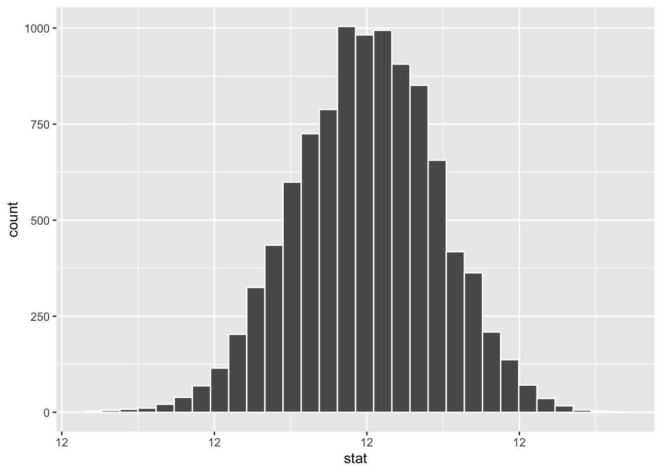
## # A tibble: 1 × 2
##   boot_dist_mean boot_dist_SE
##            <dbl>        <dbl>
## 1           12.0       0.0117
Observe that the mean of the the null_dist_bootstrap matches the null hypothesis value of 12. That’s the effect of placing hypothesize(..., mu = 12) into the bootstrap workflow. The nature of an \(H_0\)-centered Bootstrap Null Distribution is defined below.
Bootstrap Null Distribution
Bootstrapping a sample with mean \(\bar{x}\) creates with-replacement re-samples, each with its own mean. Those re-sampled means form a bootstrap distribution centered at \(\bar{x}\). A Bootstrap Null Distribution is created by shifting the bootstrap distribution left or right to be centered on the null hypothesis assumption \(\mu=\mu_0\). Thus, the resulting Bootstrap Null Distribution has the exact same standard deviation (SE) as an \(\bar{x}\)-centered bootstrap distribution.
For the current example, a bootstrap distribution generated for the purpose of a simulation-based CI would be centered on the sample mean \(\bar{x} = 11.91\) as discussed at length in Chapter 4. Moving that distribution to the right by the quantity \((\mu_0-\bar{x}) = .09\) results in the corresponding Bootstrap Null Distribution centered at \(\mu_0=12\).
The implication of a Bootstrap Null Distribution being centered upon the null hypothesis assumption is that it becomes a simulation-based probability model to judge how extreme the observed sample mean is compared to the null hypothesis. Remember, in the world of hypothesis tests, the assumption that the null hypothesis is the true state of the universe is the baseline for judging how extreme a sample is. In theory-based tests, the mathematical sampling distribution (based upon assumptions) is the judge. In simulation-based tests, a simulated \(H_0\)-centered Bootstrap Null Distribution is the judge.
The above summary and discussion of the Bootstrap Null Distribution was important in the effort to explore the concept in general, but was not needed to complete the hypothesis test. The code below uses the previously computed soda_curmudgeon sample mean \(\bar{x} = 11.91\)oz as the obs_stat (observed sample statistic).
null_dist_bootstrap %>%
  get_p_value(obs_stat = 11.91 , direction = "two_sided")
## Warning: Please be cautious in reporting a p-value of
## 0. This result is an approximation based on
## the number of `reps` chosen in the
## `generate()` step.
## ℹ See `get_p_value()`
##   (`?infer::get_p_value()`) for more
##   information.
## # A tibble: 1 × 1
##   p_value
##     <dbl>
## 1       0
Forget the warning in the output for a second. Obviously \(0<.05\), so therefore the sample supports rejecting \(H_0\) in favor of the alternative hypothesis. It’s as simple as that.
Infer Package Test Direction
The
directionvalue set in theget_p_value()function for ANY simulated Infer package hypothesis test should match the “direction” of the alternative hypothesis:
direction="two_sided",direction="less", ordirection="greater"
Now back to the warning. As discussed in Section 5.1, a theory-based p-value can never be 0 since there is always area under the tail of a T (or normal) distribution no matter how far out the test statistic might be. But a simulation-based p-value can be 0, as noted by the rather cryptic warning message. The reason for that is a Bootstrap Null Distribution is discrete (not continuous) being based on a finite number, say 10,000, of re-sample means. Thus, it’s tails have to stop somewhere and don’t go on forever towards \(\pm\infty\).
Recall that the theory-based test of the soda_curmudgeon data in Section 5.1 resulted in the p-value \(p =.000000000692\). Indeed, that would round off to 0 using the minimal accuracy (a few decimal places) required for comparison with a value such as \(\alpha=.05\).
Although not necessary to draw conclusions from a hypothesis test, the extra “visualization” functions included with Infer, such as shade_ci() introduced in Section 4.9, offer a great way to picture what’s going on. Indeed, those “visualization” functions were used to create the p-value and CI shadings in the previous section in Figures 5.5 and 5.4.
Figure 5.6 uses both shade_ci() and shade_p_value() in the same plot. We already drew a conclusion to the test above using the p-value, so the code below simply sends the computed CI to the shade_ci() for a visualization.
# Get the Simulation Based CI
ci <- null_dist_bootstrap %>%
  get_ci(level=.95, type = "se", point_estimate=11.91)
# Visualizing the test results - p-value and CI
null_dist_bootstrap %>%
  visualize() +
  shade_p_value(obs_stat = 11.91, direction = "two_sided") +
shade_ci(endpoints = ci) 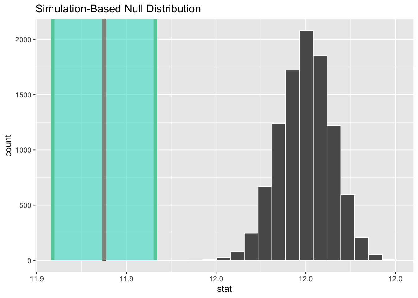
Figure 5.6: Visualizing Hypothesis Test Tesults
The vertical red line in the shade_p_value() plot on the left shows the sample mean \(\bar{x} = 11.91\) compared to the bootstrap null distribution, which is centered at the \(H_0\) \(\mu = 12\) assumption. None of the bootstrap null distribution is out as far as \(\bar{x}\) (vertical red line), so no p-value area is shaded. That’s consistent with the p-value of 0 computed further above.
The green shaded Figure 5.6 shows the 95% CI centered on \(\bar{x}\). It obviously doesn’t contain the \(H_0\): \(\mu = 12\) assumption, again consistent with the reject \(H_0\) conclusion of this test.
5.4 Random Draw Proportion Test
This section focuses on simulation-based hypothesis tests about a single-sample proportion. For an example, we’ll return to the standard 6-sided die  . The fairness of dice has long been a source of speculation. Even when manufactured carefully with consistent dimensions and density, some have speculated that the small indentations used to number a die can cause an imbalance. For example, there are 6 indented holes (or dots) on one side, and on the opposite side there is only 1 hole. It is logical to conclude that the side with only 1 hole is a bit heavier than the opposite side with 6 holes since making holes, even small ones, involves removing material. So it would not be unreasonable to conclude that the heavier side with the 1 might be more likely to land facing down, making a roll of 6 occur more often than it should.
The following hypothesis test will be used to test this conjecture, where \(p\) is the proportion of rolls that come up 6. Here p can also be thought of as simply the probability of rolling a 6, which for a fair die would of course be 1/6. Even though the conjecture is that \(p\gt1/6\), the test is formulated as two-sided to avoid biasing it in one direction. That’s a subtle point which is discussed further in Section 5.6.
| Null Hypothesis \(H_0\): | \(p=1/6\) | proportion of 6’s is 1/6 |
| Alternative Hypothesis \(H_A\): | \(p\ne1/6\) | proportion of 6’s is not 1/6 |
| Confidence Level: 95% \((\alpha = .05)\) |
To conduct the test, a die with non-numbered sides (no holes) is obtained from a company with known accuracy in manufacturing standards for dice. Holes slightly larger than usual, perhaps holes more readily visible to someone with bad vision, are carefully drilled - 6 holes one one side and 1 hole on the opposite side. No holes are drilled on the remaining sides. Instead numbers 2,3,4,5 are simply drawn on the other sides, leaving the only potential weight imbalance between the 1 and 6 sides. Numbering the other sides isn’t technically necessary for this test, but it does provide more data that could be used in additional analyses.
For the experiment, the test die is rolled 1000 times, with the result of each roll recorded in the following table imported from CSV. You can see how each roll is recorded in the die_rolls table as shown on the left. The right shows a group_by() which counts (tally()) how many times each number occurred.
die_rolls <- read_csv("http://www.cknuckles.com/statsprogramming/data/die_rolls.csv")
die_rolls

die_rolls %>%
  group_by(roll) %>%
  tally()      # Shortcut for summarize( n=n() )
## # A tibble: 1,000 × 1
## roll
## <dbl>
## 1 6
## 2 3
## 3 4
## 4 2
## 5 5
## 6 1
## 7 6
## 8 3
## 9 5
## 10 5
## # ℹ 990 more rows## # A tibble: 6 × 2
## roll n
## <dbl> <int>
## 1 1 162
## 2 2 139
## 3 3 161
## 4 4 198
## 5 5 167
## 6 6 173
For a fair die, each side is expected to come up \(1/6=0.1667\) of the time, which is about 167 times out of the 1000 rolls. The 6 side did come up more times than expected (\(\hat{p}=176/1000=.176\)). But is the difference statistically significant? The hypothesis test will answer that at a 95% confidence level.
Just like in Section 4.9, we are faced with a limitation of the specify() Infer package function in that it’s not flexible enough to specify a success condition like the following: specify(response = roll, success = "6"). The success condition must be a categorical variable with EXACTLY two values. A quick wrangle solves that problem by mutating an is_6 column with TRUE/FALSE values onto the table.
die_rolls_wrangled <- die_rolls %>%
  mutate(is_6 = (roll==6))
die_rolls_wrangled
## # A tibble: 1,000 × 2
##     roll is_6
##    <dbl> <lgl>
##  1     6 TRUE
##  2     3 FALSE
##  3     4 FALSE
##  4     2 FALSE
##  5     5 FALSE
##  6     1 FALSE
##  7     6 TRUE
##  8     3 FALSE
##  9     5 FALSE
## 10     5 FALSE
## # ℹ 990 more rows
The Infer package workflow to generate the simulation-based distribution that models the null hypothesis being true is shown below.
null_dist_draw <- die_rolls_wrangled %>%
  specify(response = is_6, success = "TRUE") %>%
  hypothesize(null = "point", p = 1/6) %>%       # The NULL HYP
  generate(reps = 10000, type="draw") %>%        # Random Draw Null Distribution
  calculate(stat = "prop")
The above code for a proportion has some noteworthy differences from that for a simulation-based test for a mean. Of course, specify() sets the Bernoulli trial success criteria as discussed above. The null hypothesize() specifies a point estimate for a proportion \(p\), and calculate() indicates that the “prop” (proportion of successes) sample statistic be calculated for each of the 10,000 re-samples in the simulation.
The three columns below show the following from left to right: the null_dist_draw simulation-based null distribution created by the Infer code above, a histogram for null_dist_draw, and finally its mean and standard deviation. Note that its mean is the same as the null hypothesis assumption of \(p=.167\) since the distribution provides a probability model that assumes the null hypothesis is true.
## Response: is_6 (factor)
## Null Hypothesis: point
## # A tibble: 10,000 × 2
##    replicate  stat
##        <int> <dbl>
##  1         1 0.168
##  2         2 0.169
##  3         3 0.166
##  4         4 0.187
##  5         5 0.183
##  6         6 0.17
##  7         7 0.191
##  8         8 0.164
##  9         9 0.165
## 10        10 0.171
## # ℹ 9,990 more rows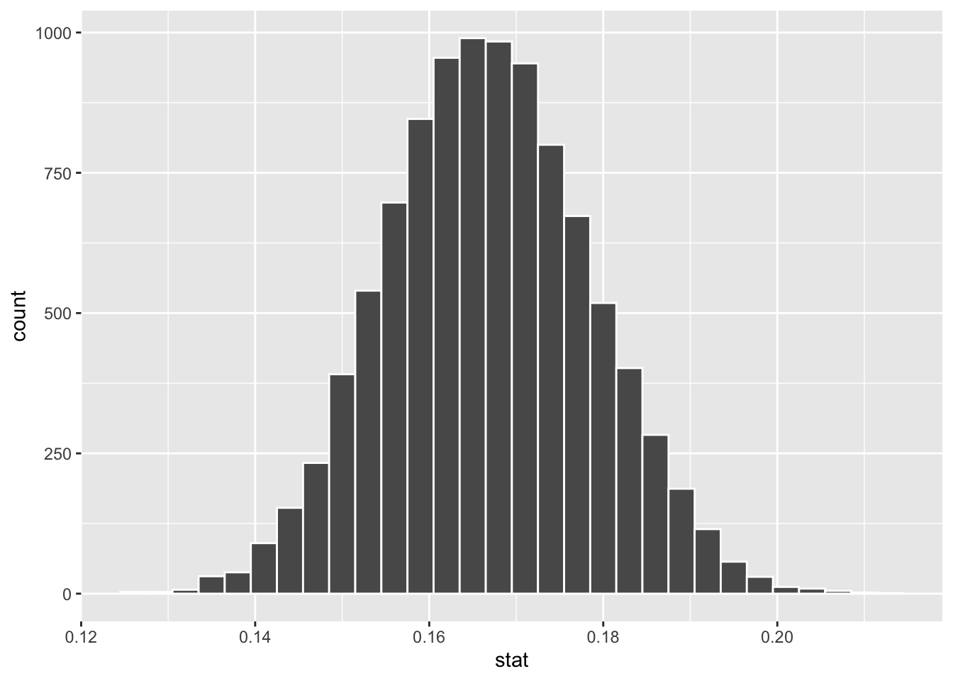
## # A tibble: 1 × 2
##   draw_dist_mean draw_dist_SE
##            <dbl>        <dbl>
## 1          0.167       0.0118
The remaining mystery about the Infer package code in this example is what generate(...,type="draw") is about, and why we used similar terminology in naming the null_dist_draw distribution. In fact, you may have noticed that mention of bootstrap is missing from this example. That’s because this simulated Null Hypothesis sampling distribution was NOT created through bootstrapping as in the previous section. It could have been, but there is a better simulation technique for single-sample proportion tests.
The null_dist_draw distribution was created through random draws from a Bernoulli experiment that matches the null hypothesis of \(p=1/6\). The original sample contains \(n=1000\) die rolls. A new size \(n\) fabricated sample can be created by simulating a sequence of 1,000 random draws (Bernoulli trials), each with probability \(p=1/6\) of success. Such a fabricated random draw sample is NOT a re-sample taken from the original sample in the sense of bootstrapping, but rather a completely new simulated sample based solely upon the null hypothesis assumption.
Fabricating 10,000 different random draw samples as described above creates a Random Draw Null Distribution that models the null hypothesis.
Random Draw Null Distribution
A simulation-based distribution of proportions that models the null hypotheisis assumption \(p=p_0\) is constructed by fabricating samples of \(n\) random draws, each draw having probability \(p_0\) of success. The samples fabricated through random draws have the same size \(n\) as the original sample. The resulting success proportions, computed from each of the random draw sample replicates, forms a simulated Null Distribution that’s centered on \(p_0\).
When the Infer package call to hypothesize() is sent the \(p\) parameter as in hypothesize(null = "point", p = 1/6)
(instead of sending a \(\mu\)), that automatically causes the generate() function to default to type="draw" (rather than bootstrap). That is, we could have simply done generate(reps = 10000) above, and type="draw" would have been used automatically since a proportion \(p\) was hypothesized. However, it’s best to explicitly specify type="draw" as we did to emphasize the nature of the simulation method being used.
The underlying concept of random draw null distributions is quite interesting so we’ll try to talk it through from another angle. A null hypothesis about a population mean, say \(\mu=12\), is just a number with no direct simulation potential. You can’t fabricate new samples that simulate having mean of 12 out of thin air from an unknown population. Hence, extra information (to model sampling variation) is coaxed out of the original sample by bootstrapping it. In contrast, a null hypothesis assumption about a population proportion, say \(p=1/6\), has direct simulation potential through Bernoulli trials. You can fabricate new simulated samples out of thin air through random draws, each with probability 1/6 of success.
Fortunately, the Infer package internally takes care of all the work to construct the 10,000 random draw samples. Using the null_dist_draw computed above, the following two blocks of code compute the p-value as shown on the left, and then visualize the p-value as shown on the right. Notice that the observed proportion \(\hat{p}=176/1000=.176\) of rolls resulting in 6 computed from the original sample is sent to both of the Infer package p-value functions below.
null_dist_draw %>%
  get_p_value(obs_stat = .176 , direction = "two_sided")

# Observed sample proportion with shaded p-value
null_dist_draw %>%
  visualize() +
  shade_p_value(obs_stat = .176, direction = "two_sided")
## # A tibble: 1 × 1
## p_value
## <dbl>
## 1 0.459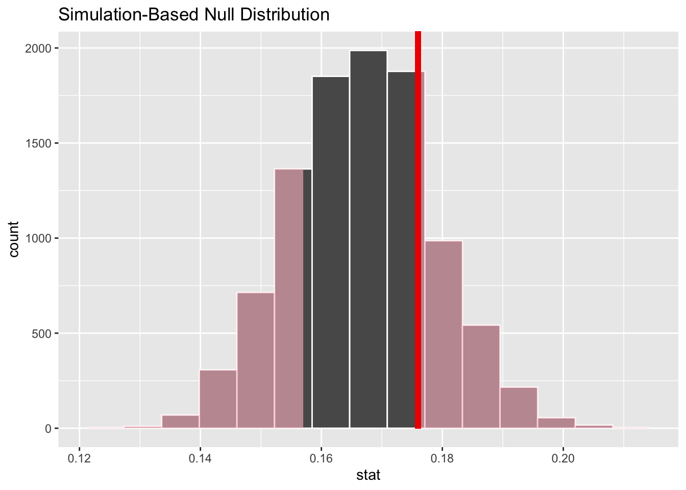
The conclusion is readily apparent since the p-value is larger than \(\alpha=.05\). The sample evidence fails to reject the null hypothesis assumption that a 6 is rolled \(1/6\) of the time. Even though a 6 was rolled 176 times in the test sample, which is 9 more times than the null hypothesis value of 167 per 1000 rolls, the difference was found to NOT be statistically significant. Essentially, swings of \(\pm9\) of one die outcome are well within the natural sampling variation that’s expected when rolling a die 1000 times.
The Infer package could be used to compute a 95% CI for this example. Of course the same conclusion would be reached, meaning the CI would contain the null hypothesis value of 167.
5.5 Permutation Difference Tests
One of the most interesting things about simulation-based hypothesis tests is the different methods used for simulating the null hypothesis. For a test about a mean, we have seen that a bootstrap distribution simulates the null hypothesis when it is shifted to be centered on the \(H_0\) assumption rather then the sample mean. For a proportion, the previous section demonstrated that random draws, each with probability of success set by the null hypothesis, are used to fabricate samples whose success proportions form a simulated null hypothesis sampling distribution.
For both types “difference of” tests - means and proportions - a third simulation method is used called Permutation Re-Sampling. Unlike bootstrap re-sampling which is with replacement, permutation re-sampling is done without replacement. You may have heard of the term permutation outside this context, which in general simply means to re-arrange things. For example, given the sequence of numbers \((1,2,3,4,5)\), the sequence \((2,4,3,1,5)\) is one of many possible permutations, or re-orderings of the sequence. For a sequence of \(n\) numbers, there are \(n!\) (\(n\) factorial) possible distinct permutations. Even for the small number like \(n=5\), there are a relatively large number \(5!=5\cdot4\cdot3\cdot2\cdot1=120\) of distinct possible arrangements of 5 objects. We won’t need to use factorials in this section, but we brought this up as a refresher in case you have learned about permutations in the past.
In statistics, a sample is just a set of numbers where the order does not matter. In set theory, \(\{1,2,3,4,5\}\) and \(\{2,4,3,1,5\}\) are both the same set. In statistics, both those sets would have the same mean and standard deviation since it doesn’t matter in which order you add up the numbers. If the set were bootstrapped, you would likely get a different set, \({1,1,3,4,5}\) for example. However, if you do a without replacement permutation re-arrangement of that set, you get the EXACT SAME set. Thus, it seems like Permutation Re-Sampling would not be very useful in statistics.
However, permutation re-sampling has a very interesting application in simulating a null hypothesis distribution for “a difference” of test. Consider the prototypical difference of means test defined below.
| Null Hypothesis \(H_0\): | \(\mu_1-\mu_2=0\) | means are the same |
| Alternative Hypothesis \(H_A\): | \(\mu_1-\mu_2\ne0\) | means are different |
| Confidence level: 95% \((\alpha = .05)\) |
The following simple example will show how permutation re-sampling simulates a null hypothesis like above. The following code defines the data, which is listed in the output on the left, and creates the boxplot shown on the right.
test_table <- tibble(
  category = c('A','A','A','A','A','B','B','B','B','B'),
  value = 1:10
)
test_table

ggplot(data = test_table, aes(x = category, y = value)) +
geom_boxplot() ## # A tibble: 10 × 2
## category value
## <chr> <int>
## 1 A 1
## 2 A 2
## 3 A 3
## 4 A 4
## 5 A 5
## 6 B 6
## 7 B 7
## 8 B 8
## 9 B 9
## 10 B 10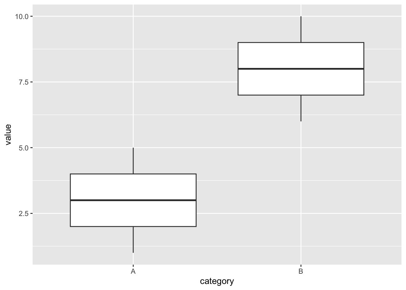
The category variable only has two categories A and B. It’s evident from the boxplots that the category A values have a mean of 3 and the category B value have a mean of 8. This is another case where you don’t need a Ph.D statistician to tell you that categories A and B have statistically different means. Clearly the above null hypothesis would be rejected. In fact, we’re not even going to run a hypothesis test on the test_table data.
The point of this example is see the effect of permutation re-sampling on the data. Since the data is rather simple, the effect will be obvious. The Infer package makes the permutation re-sampling easy. We’ll explain later what null = "independence" means in hypothesize(), but for now just focus on the fact that this code generates 10,000 permutation re-samples, three of which are shown below the code. It’s quite obvious that each permutation re-sample simply re-arranges the numbers.
permutation_re_samples <- test_table %>%
  specify(response = value, explanatory = category) %>%
  hypothesize(null = "independence") %>%
  generate(reps = 10000, type = "permute")
Three Replicates from permutation_re_samples
| category | value |
|---|---|
| A | 10 |
| A | 3 |
| A | 7 |
| A | 4 |
| A | 2 |
| B | 6 |
| B | 5 |
| B | 9 |
| B | 8 |
| B | 1 |
| category | value |
|---|---|
| A | 6 |
| A | 8 |
| A | 3 |
| A | 2 |
| A | 4 |
| B | 9 |
| B | 10 |
| B | 7 |
| B | 1 |
| B | 5 |
| category | value |
|---|---|
| A | 6 |
| A | 10 |
| A | 3 |
| A | 5 |
| A | 4 |
| B | 8 |
| B | 2 |
| B | 9 |
| B | 1 |
| B | 7 |
Forget the actual numeric values in this test data, and consider this process in a more tangible scenario. Suppose persons A and B each have 5 coins in their pocket, but person B has over twice as much money because of larger value coins. For replicate #1, they both take them out, put all of the coins in a box for a total of 10, shake the box for randomness, and then each person randomly gets 5 of the coins. Most likely, each person does not have the same coins they started with. In fact, person A could easily end up with more money than person B.
Now suppose they do this for many more repetitions, and each time persons A and B calculate the average value of the coins they end up with. Sometimes person A gets more money, sometimes person B. If they do enough repetitions, the law of large numbers says it should even out. That is, the cumulative effect of all these repetitions is that person A and person B end up getting the same amount of money on average. Symbolically, this simulates the situation of \(\mu_A=\mu_B\), or equivalently \(\mu_A-\mu_B=0\). Does that seem familiar?
Talking through the process is certainly helpful, but let’s go back to the test data and observe the actual results of the permutation re-sampling. As usual, the output of the 3 blocks of code below is organized from left to right.
# separate mean for each replicate for each category A,B
permutation_re_samples %>%
  group_by(replicate,category) %>%
  summarize( category_mean = mean(value) )

# permutation_re_samples already includes specify() %>% hypothesize() %>% generate()
perm_null_dist <- permutation_re_samples %>%
  calculate(stat = "diff in means", order = c("B", "A"))
perm_null_dist

# Handy histogram-drawing function that comes with Infer package
visualize(perm_null_dist)
## replicate category category_mean
## 1 A 5.2
## 1 B 5.8
## 2 A 4.6
## 2 B 6.4
## 3 A 5.6
## 3 B 5.4
## 4 A 6.2
## 4 B 4.8
## 5 A 5.2
## 5 B 5.8## replicate stat
## 1 0.6
## 2 1.8
## 3 -0.2
## 4 -1.4
## 5 0.6
## 6 -1.4
## 7 -0.6
## 8 -1.4
## 9 -3.8
## 10 -0.6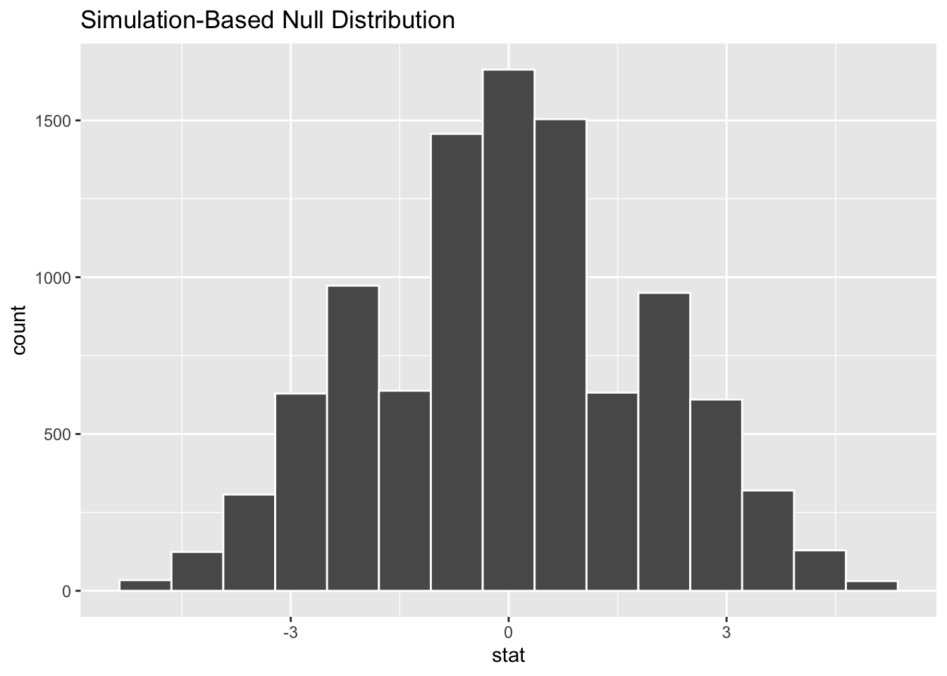
Notice in the table on the left that for each replicate, the permutation results in different means for categories A and B. In the original data, A and B had very different means. But in replicate #3, for example, the category means only differ by .2. The table in the middle was created using Infer’s calculate() function, which is much easier than computing “diff in means” with dplyr. Notice, that the “diff in means” for the replicates tend to cluster around 0. That’s further demonstrated by the histogram on the right, which is centered around 0. It was created by the handy Infer package visualize() function that plots simulated distributions with minimal code required.
The categories A and B have indeed lost their initial differences because of the permutation re-sampling. This example shows how permutation re-sampling simulates a null hypothesis of the form \(\mu_1-\mu_2=0\) that asserts there is no difference in two population means.
Recall that hypothesize(null = "independence") was specified for this simulation. Independence seems like a strange term in this context, but it makes sense if you think it through. In the case of the test data above, a null hypothesis of the form \(\mu_1-\mu_2=0\) effectively says that the response variable (numeric values) is independent of the explanatory variable (categories A and B). In short, the null hypothesis asserts that the numeric values are independent of the categories. The alternative hypothesis asserts that the two categories have different means, meaning the numeric values must somehow be dependent upon the categories.
We’ll proceed with an example using real data. Perhaps you have heard of the Internet Movie DataBase (https://www.imdb.com), which claims to be the largest free database about all things related to movies. It’s run by Amazon, so that’s a credible assertion. The ggplot2movies package comes with a very large table of data named simply movies which contains information about nearly 60,000 movies going back decades. This data used to come with the ggplot2 package to provide quick access to data for plotting examples. But the data set is so large they moved it into it’s own package named ggplot2movies to make the ggplot2 package a quicker download.
After you install and load the ggplot2movies package, at the console command line you can type movies to print the first few rows, and type ?movies to get an explanation of the nature of the data. The data contains 24 columns, some of which are have cryptic names and are not needed for this example. In order to make the data more readily viewable, the following code “slims” down the table by selecting a few of the columns. Then 10 rows (slices) are randomly selected from the slimmed down table to provide a quick looksee.
library(ggplot2movies)
# Over 58,000 movie records (rows)
movies_slim <- movies %>%
  select(title,year,length,budget,votes,rating,Action,Comedy,Drama,Romance)
# Random selection of 10 rows
movies_slim %>%
  slice_sample(n=10)
## # A tibble: 10 × 10
## title year length budget votes rating Action Comedy Drama Romance
## <chr> <int> <int> <int> <int> <dbl> <int> <int> <int> <int>
## 1 Abby 1974 89 4 e5 75 5.9 0 0 0 0
## 2 Blek Giek 2001 100 NA 16 5.4 0 0 0 0
## 3 Pasport 1990 103 NA 74 7.6 0 1 0 0
## 4 New York, New Y… 1977 163 1.4e7 1616 6.3 0 0 1 0
## 5 Hell's Kitchen 1939 81 NA 51 4.5 0 0 1 0
## 6 Remember the Ti… 2000 113 3 e7 14195 7.4 0 0 1 0
## 7 Tren del desier… 1996 27 NA 15 6.1 0 0 0 0
## 8 Loin du Bresil 1992 100 NA 6 6 0 0 0 0
## 9 Very Thought of… 1944 99 NA 55 6.3 0 0 1 1
## 10 Lethal Weapon 1987 117 1.5e7 20041 7.5 1 1 0 0The objective of this example is to perform the difference of means hypothesis test as outlined at the beginning of this section to see if the average rating of Action movies is different than the average rating of Comedy movies.
To get a meaningful comparison, we wish to only consider movies in the modern era, say after 1970 (have to go back to include Star Wars!), movies that are full-length (no short films), and movies that didn’t get many votes (the number of people that rated the movie). It’s hard to trust a rating from only a few people. The year 1970 seems reasonable for a cutoff, but to get reasonable cutoffs for the number of votes and movie length, it’s helpful to generate summaries.
summary(movies_slim$votes)
##    Min. 1st Qu.  Median    Mean 3rd Qu.    Max.
##       5      11      30     632     112  157608
summary(movies_slim$length)
##    Min. 1st Qu.  Median    Mean 3rd Qu.    Max.
##     1.0    74.0    90.0    82.3   100.0  5220.0
Observing the median and mean, the votes variable is bigtime skewed right. Around half the movies only got rated by 30 people or less. Moving up to below the mean, 500 seems a reasonable cutoff for the number of votes to make a rating meaningful. The length variable is also skewed right, but not nearly as badly. We don’t want to eliminate short movies that are still considered full-length, so 70 minutes long seems a reasonable cutoff since few modern movies are that short, and 70 is below the 1st quartile so not too many movies will get excluded. This leads to the following filter.
movies_filtered <-  movies_slim %>%
  filter(votes>=500 & year>=1970 & length>=70) %>%
  drop_na(rating)   # Obviously we don't want NA ratings
After the filter, there are still over 5000 movies left. That should provide a good basis for comparison of Action vs Comedy Ratings. The next hurdle are the genre columns in the data: Action, Comedy, etc. Unfortunately, those columns are not Tidy. Ideally, one could pivot the genre columns to create one categorical genre column containing values Action, Comedy, etc. Then it would be Tidy.
But there are two problems with that approach. First, notice that the last movie (Lethal Weapon) in the above random slice is classified as both Action and Comedy. In other words, the genre categories are not mutually exclusive in the data. So not only would a direct pivot to tidy those columns be problematic. But for a pure Action vs Comedy comparison, such multi-genre movies need to be removed.
Second, the Infer package is going to need something like specify(response = rating, explanatory = genre) where the genre column has EXACTLY two categories, in this case Action and Comedy. To overcome both of those problems, some more wrangling is in order as shown below. In the filter, we want only Action OR Comedy movies AND we do NOT (!) want dual-genre movies that are both Action AND comedy. When using complex logic, it’s best to use grouping parentheses () liberally as we have done below. The mutate then creates the genre categorical column as desired.
movies_final <-  movies_filtered %>%
  filter( (Action == 1 | Comedy == 1) & !(Action == 1 & Comedy == 1) ) %>%
  mutate(genre = case_when(
    (Action == 1) ~ 'Action',
    (Comedy == 1) ~ 'Comedy'
  ))
This results in the movies_final table we’ll use for the hypothesis test. After both rounds of filtering, we are still left with over 2,700 movies and a categorical genre column suitable to be passed into the Infer package.
That was a lot of wrangling. But in addition to being well versed in statistics, a Data Scientist simply must become comfortable manipulating the wild and crazy world of data. Sometimes you are lucky enough to find data that’s directly usable. But all too often, not so much.
Another thing a Data Scientist shouldn’t forget is the data visualization step. Before performing an inferential analysis, it’s always wise to see what you are dealing with.
# Plot of Action ratings
movies_final %>%
  filter(genre == "Action") %>%
  ggplot(mapping = aes(x = rating)) +
    geom_histogram(color = "white")

# Plot of Comedy ratings
movies_final %>%
  filter(genre == "Comedy") %>%
  ggplot(mapping = aes(x = rating)) +
    geom_histogram(color = "white")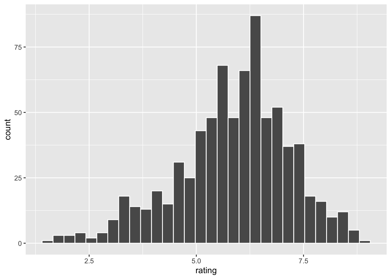
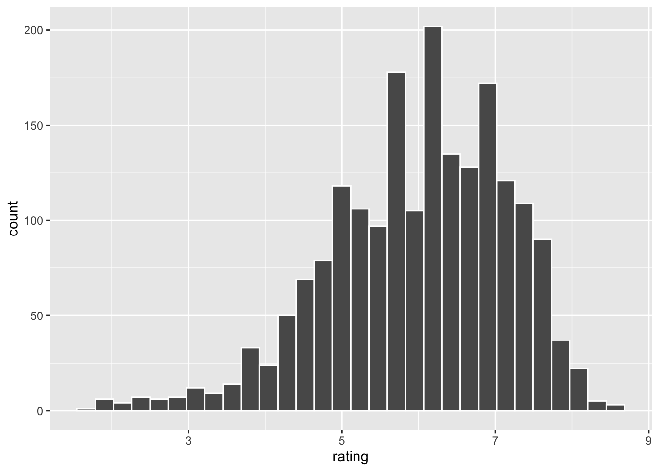
Figure 5.7: Histograms for Action and Comedy Ratings
The plots in Figure 5.7 show that both of the ratings samples are skewed but not too badly non-normal-ish. Further, both sample sizes are large and the samples are independent. So the assumptions required for a theory-based analysis of this data are probably close enough to being met that a theory-based hypothesis test would be considered reliable.
However, the samples do exhibit some skew. So many statisticians would consider a simulation-based analysis to be more appropriate in this case. The skew is also evident in the boxplots produced by the code below. The small bars on the left side of the histograms in Figure 5.7 are evident as outliers in the boxplots at the bottom of the rating scale.
# Boxplots by Genre
ggplot(data = movies_final, aes(x = genre, y = rating)) +
  geom_boxplot()

# Descriptive Stats by Genre
movies_final %>%
  group_by(genre) %>%
  summarize(n = n(), mean_rating = mean(rating), std_dev = sd(rating))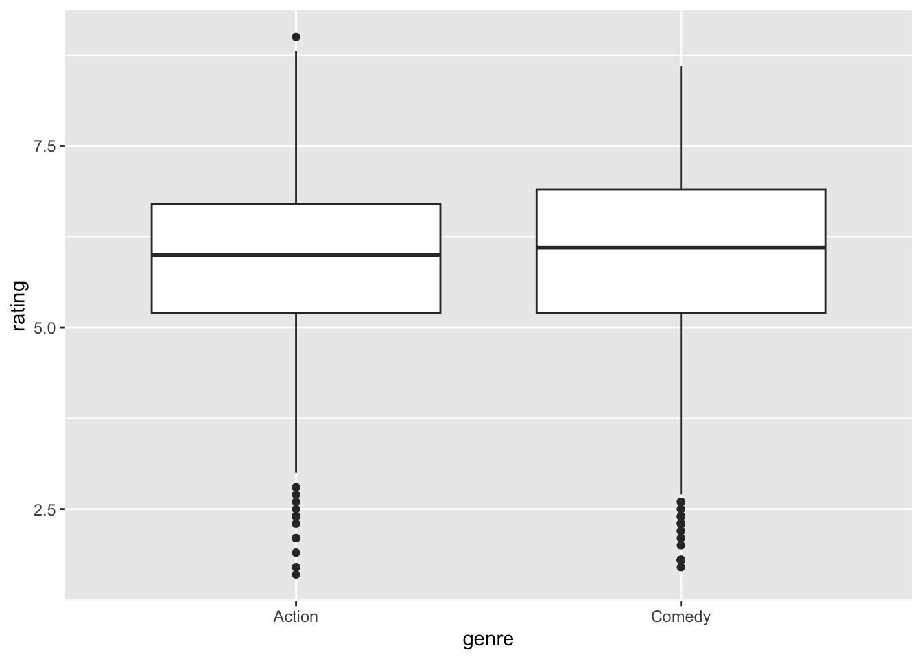
## # A tibble: 2 × 4
##   genre      n mean_rating std_dev
##   <chr>  <int>       <dbl>   <dbl>
## 1 Action   759        5.87    1.31
## 2 Comedy  1949        5.99    1.16
Visually the two samples seem very similar. Indeed, the Action and Comedy means calculated just above are surprisingly close. Since we will need the difference of means computed from the observed samples for the hypothesis test, we’ll do that below.
Having seen all this, the casual observer would probably say that the means are so close as to not be statistically different. And that’s a perfectly reasonable observation since a difference in ratings of only \(0.12\) seems small in the whole scheme of things.
However, a Data Scientist should view the situation with a bit more insight. How “close” things are in inference depends upon how wide or narrow the sampling distribution is. Recall the theory-based SE formulas for means contain fractions with sample sizes in the denominator. For this data, the sample sizes are very large, so that tends to make the SE small (big denominator) and hence a narrow sampling distribution. Large sample sizes will also tend to simulation-based distributions more narrow. The two sample means might be relatively further apart than they seem.
On the other hand, the standard deviations of the two samples computed just above are relatively large compared to the range of the data. That tends to make sampling distributions wider for both theory-based and simulation-based. So that could serve to counteract the narrowing effect of the large sample sizes. Thinking the nuances through like this is certainly insightful, but the hypothesis test will be the final judge.
The data wrangling for this analysis was a bit complicated. But with that done, completing the simulation-based hypothesis test is easily accomplished with the Infer package code below. The Infer workflow should be familiar at this point after all the previous examples, so we’ll just make a quick comment about the order specified in the calculate() function. Having observed above that the Comedy ratings had a larger mean than Action, setting the order c("Comedy", "Action") in the calculation matches the order used above to calculate the observed difference of means of \(.11634\). If the order were switched, the difference of means would switch negative to become \(-.11634\), and the hypothesis test would result in the same conclusion.
# Calculate the Simulation-Based Null Distribution
null_dist_movies <-  movies_final %>%
  specify(response = rating, explanatory = genre) %>%
  hypothesize(null = "independence") %>%
  generate(reps = 10000, type = "permute") %>%
  calculate(stat = "diff in means", order = c("Comedy", "Action"))

# Calculate p-value
null_dist_movies %>%
  get_p_value(obs_stat = 0.11634, direction = "both")

# Helpful visualization of Null Distribution and p-value
visualize(null_dist_movies) +
  shade_p_value(obs_stat = 0.11634, direction = "two_sided")
## # A tibble: 1 × 1
## p_value
## <dbl>
## 1 0.022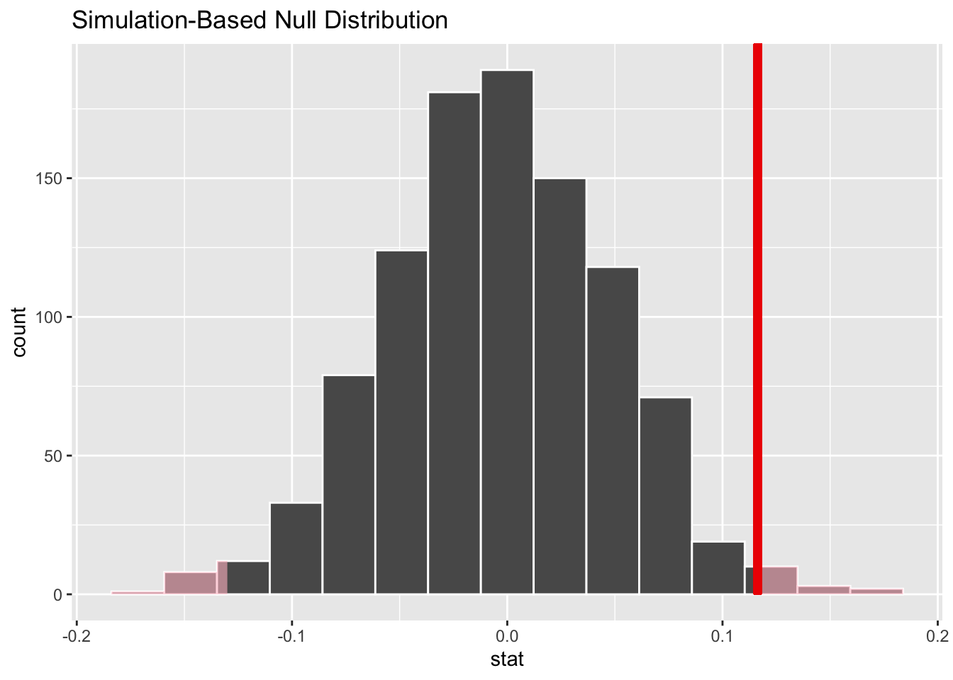
The main takeaway from the above test is that the p-value is smaller than \(\alpha\) \((.022<.05)\), so the test calls for rejecting the null hypothesis in favor of the alternative that the difference between the Comedy and Action ratings is statistically significant. Of course, the plot above with the p-value shading is not necessary to resolve the test, but does provide a helpful visualization.
Before moving on, there are two things to note about the Comedy vs Action ratings example. The first one concerns computational complexity as discussed below.
A Note about Computational Complexity
Even with modern computers, simulations can be time consuming. Because the sample sizes are so large (759 and 1949 after filtering) in the Comedy vs Action ratings example, computing 10,000 repititions takes several seconds to run on a desktop computer that’s considered relatively fast at the time this was written (3 GHz 6-Core Intel chip with lots of RAM). Also due to the large sample sizes, there was still some variablity among different runs of the 10,000 rep simulation. In such a case, the simulation-based result would be more reliable using more reps, perhaps 100,000 or a million, until the results stabilize to the desired accuracy across multiple runs. That would be readily doable on a more beefy computer system, but somewhat cumbersome on a typical desktop.
The second point is that the Comedy vs Action ratings hypothesis test wasn’t an inference about an unknown population parameter. Considering the data to be the whole known population of movies, it was testing whether a categorical difference within a known population was statistically significant. That’s a very common use for a “difference of” test, just technically not inference in the usual sense of testing a conjecture about an unknown population parameter.
This section concludes with a difference of proportions example using the same IMDB movie data that was used in the difference of means example above. Let \(p_1\) be the proportion of “low” budget movies that have a “good” rating, and \(p_2\) be the proportion of “high” budget movies that have a “good” rating. A typical difference of hypothesis test is outlined below.
| Null Hypothesis \(H_0\): | \(p_1-p_2=0\) | proportions are the same |
| Alternative Hypothesis \(H_A\): | \(p_1-p_2 \ne 0\) | proportions are different |
| Confidence level: 95% \((\alpha = .05)\) |
The data wrangling required to prepare the data actually involves more work than using the Infer package to run the test. To understand the nature of the needed wrangling, it’s helpful to take a look at the Infer package code below. As you can see, it’s very similar to the code used for the difference of means test above.
null_dist_movie_budget <- movies_data_categorical %>%
  specify(response = rating_level, success = "Good_Rating", explanatory = budget_level) %>%
  hypothesize(null = "independence") %>%
  generate(reps = 10000, type = "permute") %>%
  calculate(stat = "diff in props", order = c("High_Budget","Low_Budget"))
Like with means, the permutation simulation method is used for the “diff in props” test. The Infer package requires the explanatory variable to be categorical with exactly two values (same requirement for a “diff in means” test). But for a proportion test, the response variable must also be categorical with exactly two values, one of which indicates success, so that the proportion of successes can be computed for each simulation replicate.
However, the IMDB movies data is not structured that way. Both the movie ratings and the movie budgets are numbers. Those columns will need to be wrangled into two-value categorical variables. We’ll start with the same filter used before to eliminate old, short, and movies with unreliably few ratings. This time we drop any movie records that have a NA rating OR budget. Quite a few movies in the original data don’t list a budget.
movies_with_budget <-  movies %>%
  filter(votes>=500 & year>=1970 & length>=70) %>%
  drop_na(rating,budget)

summary(movies_with_budget$rating)
##    Min. 1st Qu.  Median    Mean 3rd Qu.    Max.
##    1.70    5.40    6.30    6.19    7.10    9.10
summary(movies_with_budget$budget)
##     Min.  1st Qu.   Median     Mean  3rd Qu.     Max.
## 0.00e+00 6.00e+06 1.70e+07 2.72e+07 4.00e+07 2.00e+08
The summaries above are helpful in creating the needed two-value categorical variables since we need some notion of low/high budget and bad/good rating. We’ll use the medians as the low/high and bad/good cutoffs. That’s an arbitrary choice, but it is logical to use the middle numeric values to create two-value categories.
The code below does the required wrangling, selects the relevant columns to slim down the table, and then grabs a random slice_sample so we can take a looksee at the result. We used extra-descriptive categories such as ‘High_Budget’ just to make things more human readable, which is always a good programming practice.
movies_data_categorical <- movies_with_budget %>%
  mutate(
      rating_level = case_when(
        (rating >= 6.3) ~ 'Good_Rating',
        (rating < 6.3) ~ 'Bad_Rating'
      ),
      budget_level = case_when(
        (budget >= 17000000) ~ 'High_Budget',
        (budget < 17000000) ~ 'Low_Budget'
      )
  ) %>%
  select(title,rating_level,budget_level)

movies_data_categorical %>%
   slice_sample(n=10)
## # A tibble: 10 × 3
##    title                                 rating_level budget_level
##    <chr>                                 <chr>        <chr>
##  1 1900                                  Good_Rating  Low_Budget
##  2 Harry Potter and the Sorcerer's Stone Good_Rating  High_Budget
##  3 Bridges of Madison County, The        Good_Rating  High_Budget
##  4 Matrix Reloaded, The                  Good_Rating  High_Budget
##  5 Garage Days                           Bad_Rating   Low_Budget
##  6 Drive                                 Good_Rating  Low_Budget
##  7 Apt Pupil                             Good_Rating  Low_Budget
##  8 Legal Eagles                          Bad_Rating   High_Budget
##  9 Trancers                              Bad_Rating   Low_Budget
## 10 Mallrats                              Good_Rating  Low_Budget
Before running the hypothesis test, as always it’s a good idea to explore the data a bit as shown in the barplot in Figure 5.8.
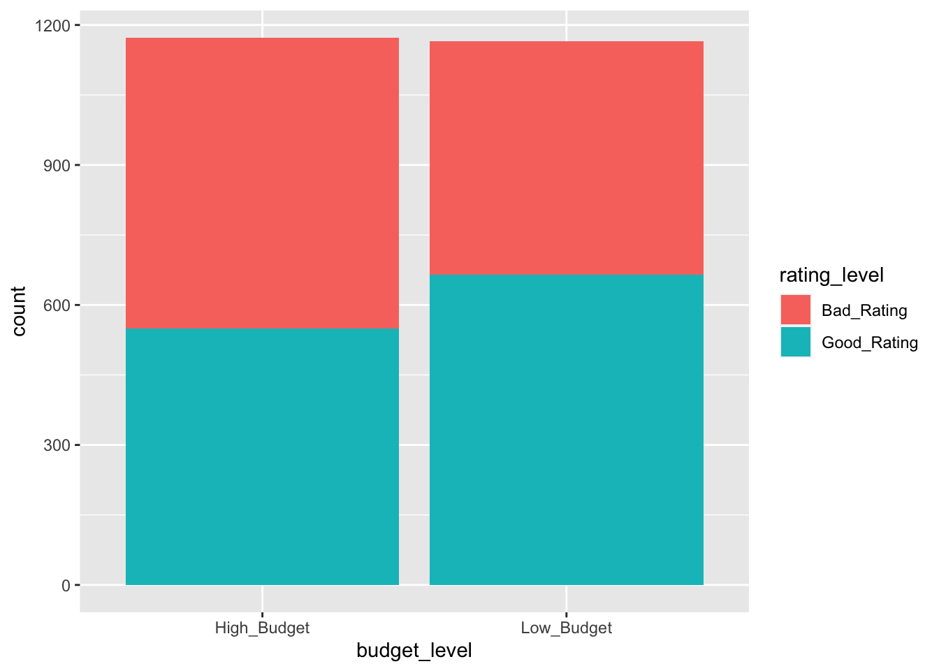
Figure 5.8: Rating Proportions by Budget Level
Visually it’s obvious that less than half the high budget movies have good ratings, but more than half of the low budget movies have good ratings. To compute the difference of proportions we’ll use the same Infer package code that was shown near the beginning of this example, just leaving out the simulation parts. That’s a technique that’s been used in a few prior examples.
movies_data_categorical %>%
  specify(response = rating_level, success = "Good_Rating", explanatory = budget_level) %>%
  calculate(stat = "diff in props", order = c("High_Budget","Low_Budget"))
## Response: rating_level (factor)
## Explanatory: budget_level (factor)
## # A tibble: 1 × 1
##     stat
##    <dbl>
## 1 -0.102
From the order specified in the calculate() function, the negative result quantifies the barplot visual that low budget movies have a larger proportion of good ratings. Go figure. In fact, the difference in proportions is over 10%. At this point it seems that the hypothesis test will find the proportions to be significantly different.
To the end, it’s time to run the Infer package code shown near the beginning fo this example to create the null_dist_movie_budget as it’s named there. Since we showed the code above, we won’t show it again here. But assume at this point that the simulation-based null_dist_movie_budget has been computed.
Using that an the difference in proportions computed above, the p-value is easily calculated using the Infer package.
null_dist_movie_budget %>%
  get_p_value(obs_stat = -.102, direction = "both")
## Warning: Please be cautious in reporting a p-value of
## 0. This result is an approximation based on
## the number of `reps` chosen in the
## `generate()` step.
## ℹ See `get_p_value()`
##   (`?infer::get_p_value()`) for more
##   information.
## # A tibble: 1 × 1
##   p_value
##     <dbl>
## 1       0
The null hypothesis is soundly rejected in favor of the alternate hypothesis that the proportion of movies rated highly is different for low and high budget movies.
It’s important to remember that p-values of 0 can occur in simulation-based tests since the null distribution is discrete. However, in theory-based tests the distribution (T or Z) of the test statistic is continuous, so there is always some tail area no matter how far out toward \(\pm\infty\) the test statistic falls in the tail. A corresponding theory-based two-sided 95% test results in a test statistic value of \(z=-4.96\), which results in a p-value of approximately \(p=.0000007\) giving the same result.
Assumptions
The previous paragraph compared the theory-based result (\(p=.0000007\)) to the simulation-based result (\(p=0\)). It is IMPORTANT to note that the data in this example satisfies the assumptions listed in Section 4.4 required by the mathematics behind the theory-based difference of proportions formulas. Those assumptions are not required for a simulation-based test, but one should never forget that theory-based tests are dependent on assumptions.
As a final note in this section, the purpose of the previous example was to show the use of the Infer package to conduct a difference of proportions test. Although the test (and data wrangling) was interesting, the “diff in props” analysis wasn’t necessarily the best statistical approach to use to explore the relationship between movie budget and ratings. Indeed, a linear regression analysis to explore the actual numerical relationships between movie budget and rating would provide more perspective than simply dividing the numerical data into categories for the proportion analysis.
5.6 Hypothesis Test Subtleties
We have saved some of the most subtle details and nuances about hypothesis tests for the final section of this chapter because we didn’t want to obscure the main concepts and computational techniques presented in the previous sections. The examples and insights already discussed in this chapter provide a solid foundation from which to understand some of the more subtle nuances about hypothesis tests. Some of those subtleties have already been mentioned briefly or foreshadowed, but more details are presented below.
5.6.1 Choice of Confidence Level
The choice of a confidence level often seems arbitrary when first learning statistics. Why not always just choose something like 99% or 99.9% so that you are supremely confident in the result? Well, it’s not quite that simple. For starters, Section 4.1 discussed that higher confidence levels produce wider confidence intervals, hence less precise interval estimates for unknown population parameters. A 100% confidence level is actually not useful at all since it results in a CI of \((-\infty,\infty)\) which covers the whole real number line.
That type of give and take in terms of higher confidence vs less precise estimates is evidenced by the two types of errors associated with hypothesis tests.
Error Types for Hypothesis Tests
- Type I Error - False Positive
The Null Hypothesis is True, but you reject it based on the sample.- Type II Error - (False Negative)
Null Hypothesis is False, but you fail to reject it based on the sample.
An unknown population parameter is a number that exists in nature or in the universe, but you just don’t know what it is. The null hypothesis is therefore either true or false, you just don’t know which. Hence, you take a sample and do a statistical analysis. It’s basically a game of chance. Either type of error described above can happen if you get an “unlucky” (non-probable) sample that doesn’t represent the population very well.
Consider a pharmaceutical company testing a new drug that they hope passes some threshold - the alternative hypothesis - to get approved for use. The status quo - the null hypothesis - is that it doesn’t. In a Type I error, it would be true that the new drug doesn’t work, but because of some unlucky testing it gets approved for use - a false positive. In a Type II error, it would be true that the new drug really does work, but because of some unlucky testing it gets rejected for use - a false negative. Which is better?
Approving an ineffective drug to treat life threatening conditions is clearly bad, especially if there is another drug that could provide at least some benefit. But so is failing to approve a new drug that could actually save lives when other drugs aren’t very effective. It really depends upon the situation. Sometimes times there is no right answer.
For a more general analogy, in a court of law is it better to convict an innocent person (false positive) or to acquit someone who actually committed the crime (false negative). Someone might say that it’s better to let a guilty person go free than to imprison an innocent person. Sounds logical, right? But what if the guilty person that goes free commits additional horrible crimes? Again, it really depends on the specifics of the situation, and there may be no right answer.
In the guilty/innocent analogy, a civilized and just society always tries minimize both types of error. But it’s not so simple in the world of statistics where it’s a game of chance, rather than logic and facts that hopefully prevail in the court room.
Type I vs Type II Errors
Mathematically, Type I and Type II errors are inversely related - when one goes down, the other goes up. It’s mathematically impossible for them to both be 0. Increasing the confidence level lowers the probability of a Type I error, but increases the probability of a Type II error.
So in some cases, it might be appropriate to use a 99% or 99.9% confidence level to help mitigate Type I errors. In other cases, it might be appropriate to use a 90% confidence level to help mitigate Type II errors. The 95% level is used most often since it strikes a nice balance in many cases. The nature of the analysis often determines the confidence level. For example, the US FDA (Food and Drug Administration) sets guidelines for different types of statistical analyses you would have to submit to get a new drug approved. Depending upon several factors, you would have to use a certain confidence level or they might not even consider a certain submission for approval. In other cases, like studies in the social sciences, it might simply be the common practice for professional journals to use a certain confidence level (e.g.95%).
But one thing is certain. The confidence level should be pre-determined based upon tradition, the type of statistical analysis, tolerance for certain types of errors, or even government guidelines that you may or may not agree with. It is considered bad statistical practice (and in some cases unethical, or even illegal) to change the confidence level to achieve a desired outcome after computing the p-value. You shouldn’t move the goalposts after taking the sample and doing the analysis.
5.6.2 Interpreting the p-value
The p-value is the probability that any sample will be at least as extreme - assuming the null hypothesis is true - as the observed sample. Basically, how likely it is that your sample data could have occurred in a universe where the null hypothesis is the true state of nature.
This seems to be one of the hardest concepts to grasp for beginning statistics students. It is somewhat of a convoluted definition that’s hard to explain. Misconceptions are common, even for people who should know better.
Common Misconceptions about p-values
- A p-value is NOT the probability that the null hypothesis is true or that the alternative is false.
- A low p-value (less than \(\alpha\)) does NOT prove that the null hypothesis is false. Rather that the null hypothesis is “probably false” based upon the observed sample data: meaning it actually is false, or it’s true but a highly improbable sample that defies the population has occurred.
5.6.3 One-Sided vs Two-Sided Tests
Examples in Section 5.1 showed that the p-value for a one-sided test is exactly half of the p-value of a corresponding two-sided test. This is true in general. For a right-sided test like below
\(H_0\): \(\mu <= 12\), \(H_A\): \(\mu > 12\)
the p-value area is entirely within the right tail of the distribution. Switch to a two sided test
\(H_0\): \(\mu = 12\), \(H_A\): \(\mu \ne 12\)
and the p-value area would double since area in the other tail would have to be included.
Thus, at a given confidence level (say 95%) it is easier to reject the null hypothesis in favor of the alternative when using a one-sided test. The claim a study seeks to validate is usually set up as the alternative hypothesis, which requires strong evidence (\(p\leq\alpha\)) to accept. A one-sided test does not require that the evidence be as strong, thereby making it easier for researchers to validate claims.
So why not always use one-sided tests when reasonable, giving you a greater chance of substantiate a claim? First, you often don’t know in advance how your sample statistic (mean, proportion, etc) is going to compare (greater or less) to the unknown population parameter, so you wouldn’t know which one-sided test to do (left or right). After observing the sample data and determining that, it would not be sound statistical practice to change the test. You shouldn’t change the the type of test (or the confidence level) after analyzing the sample to get the result you desire.
Second, two-sided tests are symmetric which makes for more of an unbiased approach - both directions provide equal evidence against the null hypothesis so that neither direction is favored. An investigator should have a valid reason for choosing a one-sided test over a two-sided one in order to steer away from bias in test. Such reasons do exist. For example, it’s common in threshold (boundary) situations, where the consideration in question is inherently one-sided. In toxicity testing, one usually only cares if the toxin level exceeds (statistically significantly, of course) some pre-set maximum contaminant level. One might want to test if a more expensive drug is more effective on average than a cheaper one, not really caring about the other direction because, if not, people would still use the cheaper one.
Correcting Directional Bias
To avoid directional bias in a one-sided test, it is sound statistical practice to increase the confidence level accordingly. For example, a 95% (\(\alpha=.05\)) two-sided test is probalistically similar to a 97.5% (\(\alpha=.025\)) one-sided test. The p-value computed for the one-sided 97.5% test will be half of the p-value computed for the two-sided 95% test, giving the same likelihood of rejecting the null hypothesis when the p-value is compared to \(\alpha\).
The bottom line is that in general you should use two-sided tests to avoid directional bias, unless there is a compelling reason to set it up as a one-sided test. And in that case, one might consider adjusting the confidence level accordingly. And finally, it’s hard to emphasize enough that you should never move the goalposts (type of test or confidence level) after observing the sample sample data to change the result.
5.7 Resources
The R scripts provided below contain code from the main examples featured in this chapter. The scripts are numbered to keep them organized in roughly the same order that the examples were presented. The script numbers do not correspond to section numbers within this chapter.
Download a Zip archive containing all the scripts listed below:
Click on Script for Source Code: