Chapter 2 Probability Distributions

The following packages are required for this chapter.

library(tidyverse)
# Tidyverse is only needed for the plots in Section 2.7.
# All the other functions featured in this Chapter are Core R (no package needed). 

This chapter explores terms and concepts related to basic probability theory and probability distributions. Extra detail is provided on Binomial distributions and Normal distributions since they are particuarly relevant in the next chapter on Sampling Theory. Throurought this chapter, the P-Q-R-D probability distribution functions are emphasized for various types of probability calculations that will be used in subsequent chapters.

2.1 Probability Terminology

A random experiment, such as flipping a coin or selecting a lottery ball, has an unknown outcome. The set of all possible outcomes of a random experiment is the sample space, often denoted by \(S\). For example, the sample space for the random experiment of rolling a standard 6-sided die is \(\{1,2,3,4,5,6\}\).

An event \(E\) is a subset of a sample space. In a random experiment, the probability of an event \(E\subseteq S\) occurring is denoted by \(P(E)\).

Basic Probability Rules:

• \(0 \le P(E) \le 1 \;\) for any event E. (Probabilities are numbers between 0 and 1, inclusive.)
• \(P(\emptyset) = 0 \;\;\) (Probability of an impossible event (empty set) is 0.)
• \(P(S) = 1 \;\;\) (Probability of a certain event (whole sample space) is 1.)

It’s sometimes convenient for humans to think of a probability as a percentage, 50% or 100% for example, but the mathematics of probability theory require the corresponding numeric values .5 or 1, respectively.

A Random Variable stands for any possible outcome of a random experiment. Random variables are often represented by upper-case letters such as \(X\), \(Y\), \(Z\). Events are often described using random variables instead of as sets. For example, the probability of the event or rolling a 1 with a standard 6-sided die is \(P(X=1) = 1/6 = .1666667\) where the random variable \(X\) represents possible outcomes. Using set-theoretic notation, the same expression becomes \(P({1}) = .1666667\).

A simple event is a single outcome in a sample space such as \(X=1\) for a die roll. A compound event involves two or more simple events such as \(X=1 \; or \; X=2\) for a die roll. Of course, \(P(X=1 \; or \; X=2) = 1/3\). However, \(P(X=1 \; and \; X=2) = 0\) since the outcome of one roll of a die can’t be both 1 and 2. The rules for compound probability calculations can be a bit tricky and are generally covered in detail in an Introduction to Statistics course, but such rules are beyond the scope of this discussion.

2.2 Discrete Probability Distributions

A probability distribution gives the probabilities for all possible outcomes for a random experiment. When the sample space of the experiment is finite, the probability distribution is called discrete and gives the probability of each simple event (individual outcome).

For example, two discrete probability distributions for rolling a die (or 2 dice) are shown in Figure 2.1.

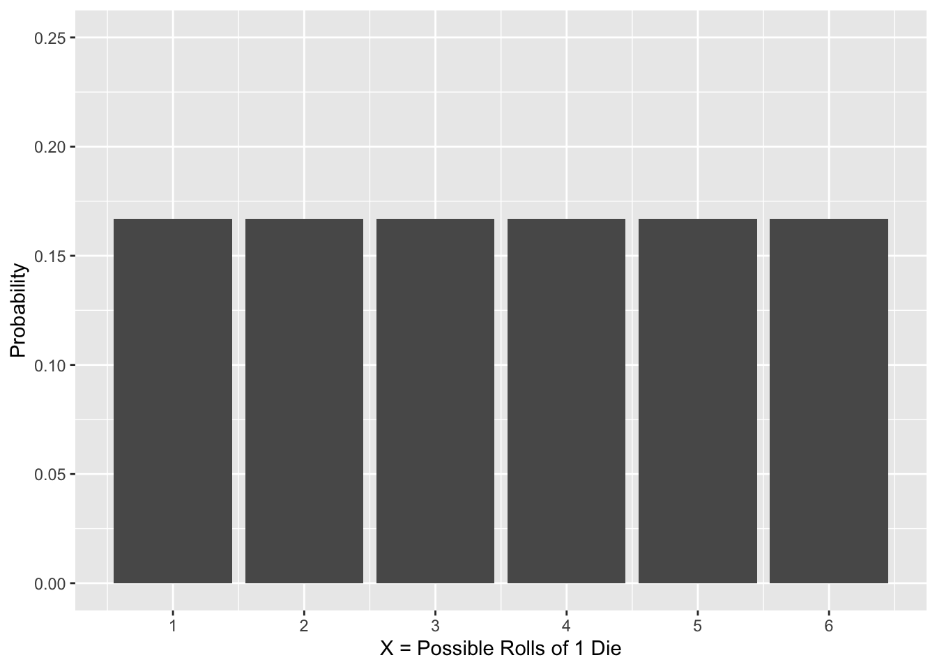
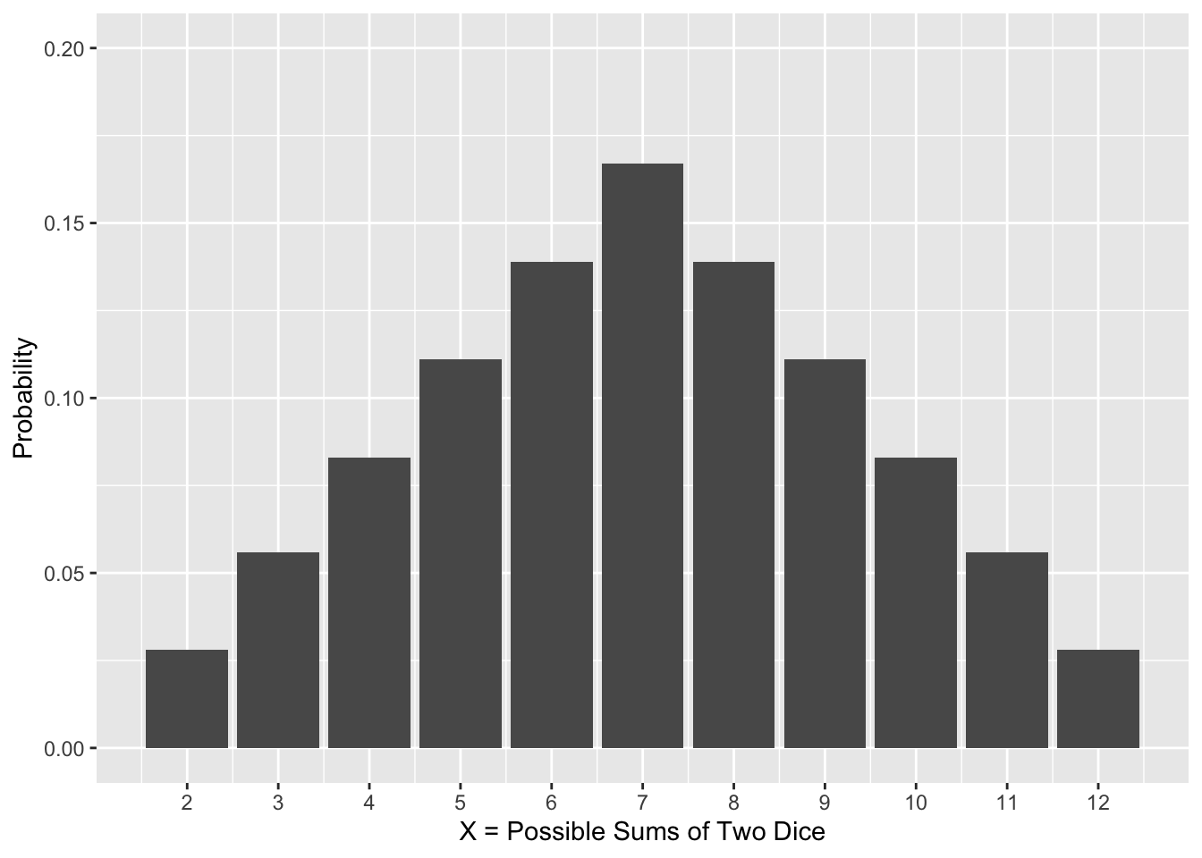
Figure 2.1: Discrete Probility Distributions

On the left in Figure 2.1, the 6 possible outcomes for rolling 1 die are listed on the x-axis and each probability on the y-axis. This is an example of a uniform distribution since each outcome has the exact same probability (assuming the die is fair and balanced, of course). The probability of a simple outcome is simply the height of the bar (\(P(X=1) = 1/6\)). The probability of a compound event is the sum of the heights of the simple outcomes (\(P(X \le 3) = 1/6 + 1/6 + 1/6 = .5\)).

The distribution on the right in Figure 2.1 models the random experiment of rolling 2 fair dice and adding the values, such as when playing the classic Monopoly board game or the popular Craps casino game. Obviously, this distribution is not uniform. But it is symmetric. The 11 possible sums are listed on the x-axis. Suppose one die is red and the other is blue and a roll is denoted by \((red,blue)\). Then a sum of 3 can result from either a roll of \((1,2)\) or \((2,1)\), giving a probability of \(P(X=3)=2/36=0.055\) since there are a total of \(6\times6=36\) distinct \((red,blue)\) ordered pairs.

Properties of Discrete Distributions:

• The x-axis lists each possible outcome of an experiment.
• The bar height for each outcome is the probability of that outcome occruring.
• The sum of all the bar heights is 1 since it’s certain that of the possible outcomes must occur.

The mean of a probability distribution, denoted by \(\mu\), is also called the expected value or simply expectation. What do you expect when you roll 2 dice and add them? The best guess (expectation) is \(\mu=7\) since that’s the most probable outcome. Or thinking of it another way, if you repeat the experiment a large number of times, say 1000 or 10,000 times, the average outcome from all those repetitions should be about \(\mu=7\). That makes sense since the distribution for the sum of two dice is symmetric meaning a sum below 7 is equally likely as a sum above 7.

The mean of a discrete distribution might not even be one of the possible outcomes. For example, the mean of the uniform distribution on the left in Figure 2.1 is \(\mu=3.5\). What’s the expected average of all the outcomes if the die is rolled 1000 times? The answer is of course 3.5, even though that’s not a possible outcome of a single roll.

Visual Interpretation of a Discrete Distribution Mean:

The mean of a discrete probability distribution can be thought of as the x-axis fulcrum (balancing point) that would balance the distribution if the probabilities are thought of as physical weights of the bars. The fulcrum is exactly in the “middle” if (and only if) the distribution is symmetric.

2.3 Binomial Distributions

Not all discrete probability distributions are symmetric. Binomial Distributions provide an such an example. Before introducing the terminology necessary to define binomial distributions in general, we’ll proceed with two easily understood examples that are depicted in Figure 2.2.

The left shows the binomial distribution resulting from flipping a fair coin 15 times and recording the number of heads that occur. The possible outcomes are \(\{0,1,2, ... ,14,15\}\).

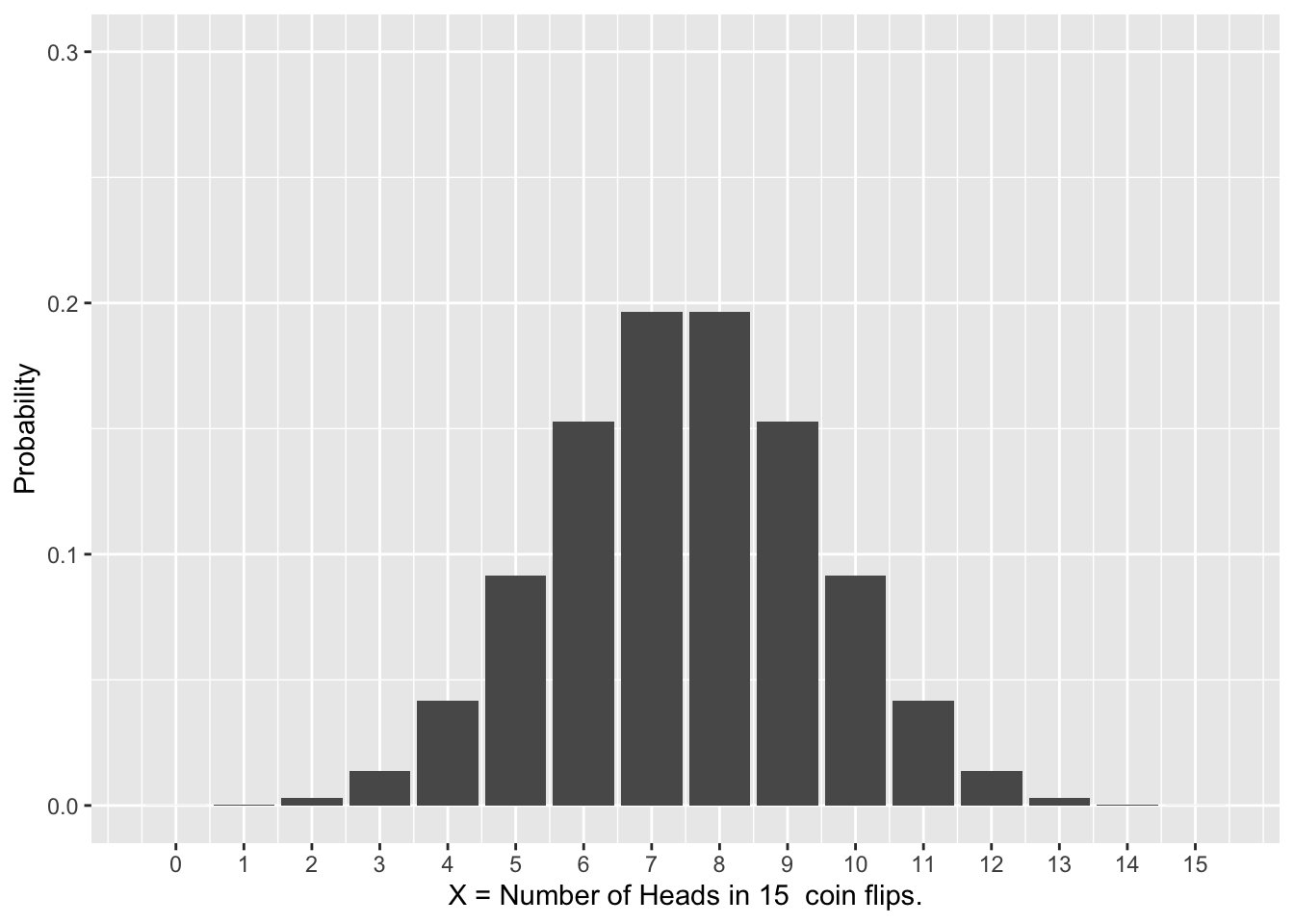
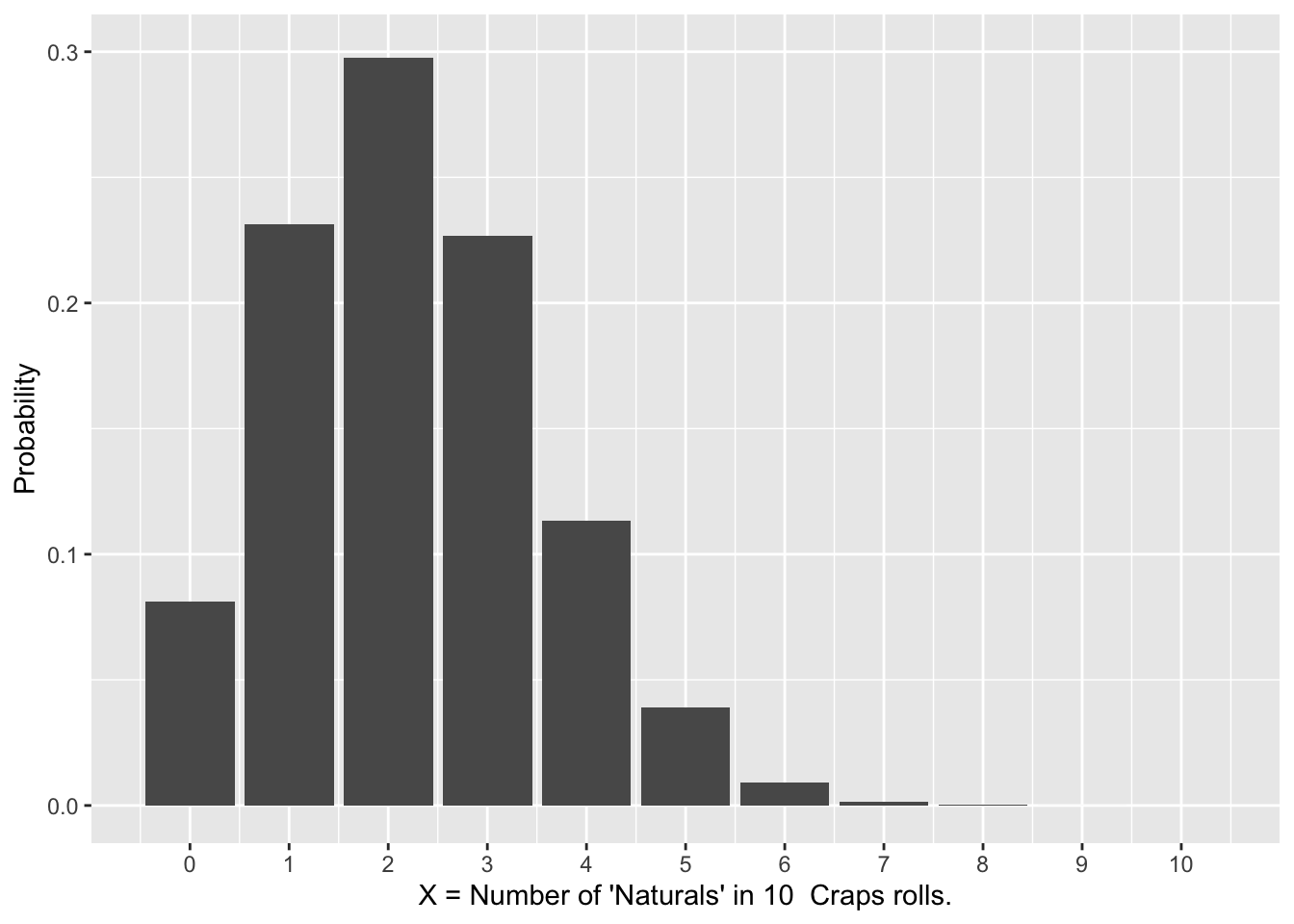
Figure 2.2: Binomial Probability Distributions

The right side of Figure 2.2 shows the binomial distribution resulting from 10 different rolls in the casino game Craps (sum of 2 dice) and recording the number of “Naturals” rolled. In craps, rolling a 7 or 11 is called a “Natural” whereas rolling a 2,3, or 12 is called “Crapping Out” (literally the roll was Crap!).

From Figure 2.2 you can see that some binomial distributions are symmetric, while others are very much not symmetric. But the bars always add up to 1. In order to explain the above distributions, we must delve into some underlying terminology.

Named after a famous mathematician, a Bernoulli Trial is an experiment that has only two outcomes: success or failure. The probability of success in a single trial is denoted by \(p\). The probability of failure is then \(1-p\) (sometimes denoted as \(q=1-p\)). Either success or failure is certain in a Bernoulli Trial since probabilities \(p\) and \(1-p\) add up to 1. Flipping a coin (success of heads is \(p=.5\)) and rolling a die (success of rolling a 1 is \(p=1/6\)) are examples of Bernoulli Trials.

A Binomial Experiment is a sequence of \(n\) independent Bernoulli Trials, each with the same probability \(p\) of success. Independence is important: the probability of success in one trial is not influenced in any way by any other trials. Probabilities for a binomial experiment are modeled by a Binomial Distribution.

The terminology for a binomial experiment is as follows. Let \(n\) be the number of independent Bernoulli trials and \(p\) the probability of success on a single trial. Then a discrete binomial distribution, denoted \(bin(n,p)\), gives the probability model for the number of successes \(x\) among the \(n\) trials. The possibilities for \(x\) are \(0,1,...,n\). For each \(x=0,1,...,n\), on the x-axis, the corresponding bar of the binomial distribution gives the probability of exactly \(x\) successes among the \(n\) trials.

Recall Figure 2.2, which shows two different binomial distributions. The distribution for the number of successes (heads) in 15 flips of a fair coin is \(bin(15,\;.5)\). The distribution for the number Naturals (sum of 7,or 11) in 10 craps rolls is \(bin(10,\;.222)\). For the craps Natural rolls \(p=8/36=.222\) since there are 8 possibilities \(\{(1,6),(6,1),(2,5),(5,2),(3,4),(4,3),(5,6),(6,5))\}\) out of 36 total that result in a Natural.

The next question is what is the expectation (mean of the distribution) for each of these binomial distributions. You can see in Figure 2.2 that the coin flips \(bin(15,\;.5)\) distribution is symmetric, so the mean would be exactly in the middle to balance it, hence \(\mu=7.5\). But the distribution for the Craps Natural rolls is very much non-symmetric. The fulcrum to balance it looks to be around 2 or 3, give or take, but we need a mathematical formula to calculate it precisely.

The values that quantify characteristics of a probability distribution are called Parameters.

Parameters of a \(bin(n,p)\) Binomial Distribution:

Parameter	Value
Mean (\(\mu\))	\(\mu=np\)
Standard Deviation (\(\sigma\))	\(\sigma=\sqrt{np(1-p)}\)

The formula for the mean makes perfect sense if you think about it: if you do the trial \(n\) times, each with \(p\) probability of success, the expectation is \(np\) successes. The Standard Deviation is a measure of the the distribution’s “spread” (how narrow or wide). The square of the standard deviation \(\sigma^2\) is called the Variance of the distribution. Both essentially measure the same thing, with the term variance being more indicative of measuring the spread (how much it varies) of the distribution.

The mean of the \(bin(15,\;.5)\) distribution (number of heads in 15 coin flips) is \(\mu=15\times.5=7.5\), a value we had already deduced above from the symmetry of the distribution. The mean of the \(bin(10,\;.222)\) distribution is \(\mu=10\times.222=2.22\). That is, you expect to get 2.2 Natural’s on average when you do 10 craps rolls. The formulas and computed values for the standard deviations are less intuitive, so we’ll pass on that for now. Much more will be said about the role standard deviations soon enough.

Skew in Binomial Distributions:

A \(bin(n,p)\) distribution with \(p=.5\) is precicely symmetric - probability of success equals the probability of failure: \(p\;=\;1-p\). If \(p\) is merley close to \(.5\), the distribution is approximately symmetric. The further \(p\) is from \(.5\), the more more skewed (non-symmetric) the binomial distribution is. If \(p\) is close to 0 or 1, the distribution is highly skewed.

It’s worth noting that if \(p\) (probability of success in one trial) is close to 0 or 1, then \(1-p\) (probability of failure in one trial) must also be close to 0 or 1. For example, if \(p=.9\) then \(1-p=.1\). Thus, if the roles of success and failure are switched (\(bin(n,p)\) to \(bin(n,1-p)\)), the resulting distribution is equally skewed, just in the opposite direction (mirror image).

To calculate binomial probabilities we first turn to mathematics. For each \(x=0,1,...,n\), the probability of exactly \(x\) successes among the \(n\) trials in a \(bin(n,p)\) experiment is given by the following formula

\[P(x) = C(n,x)\times p^x\times (1-p)^{(n-x)}\]

where \(C(n,x)=\frac{n!}{x!(n-x)!}\) is the combination of \(n\) objects taken \(x\) at a time (number of distinct subsets of size \(x\) taken from \(n\) objects).

The above formula gives the exact height of each bar in a binomial distribution. For example, the R code below calculates the exact height of the \(X=4\) bar in the \(bin(10,\;.222)\) for the number of Naturals rolled in a sequence of 10 craps rolls.

choose(10,4)*(.222)^4*(1-.222)^6   # P(X=4) for bin(10,.222)
## [1] 0.113112

Notice that the core R choose() function was used in the above calculation. The name of that function comes from the fact that \(C(n,x)\) is usually referred to as simply “n choose x.”

The above calculation can also be accomplished using the Core R pbinom() (probability binomial) function rather than the formula above. However, one first has to understand exactly what pbinom() calculates. Consider the code and its output below.

pbinom(4, size=10, prob=.222)   # P(X≤4) for a bin(10,.222) distribution
## [1] 0.9503858

Notice that we didn’t get the same value that the math formula produces. That’s because the pbinom() function computed the blue-colored left tail probability \(P(X\le4)\) (sum of all bars \(\le4\)) as shown on the left in Figure 2.3.

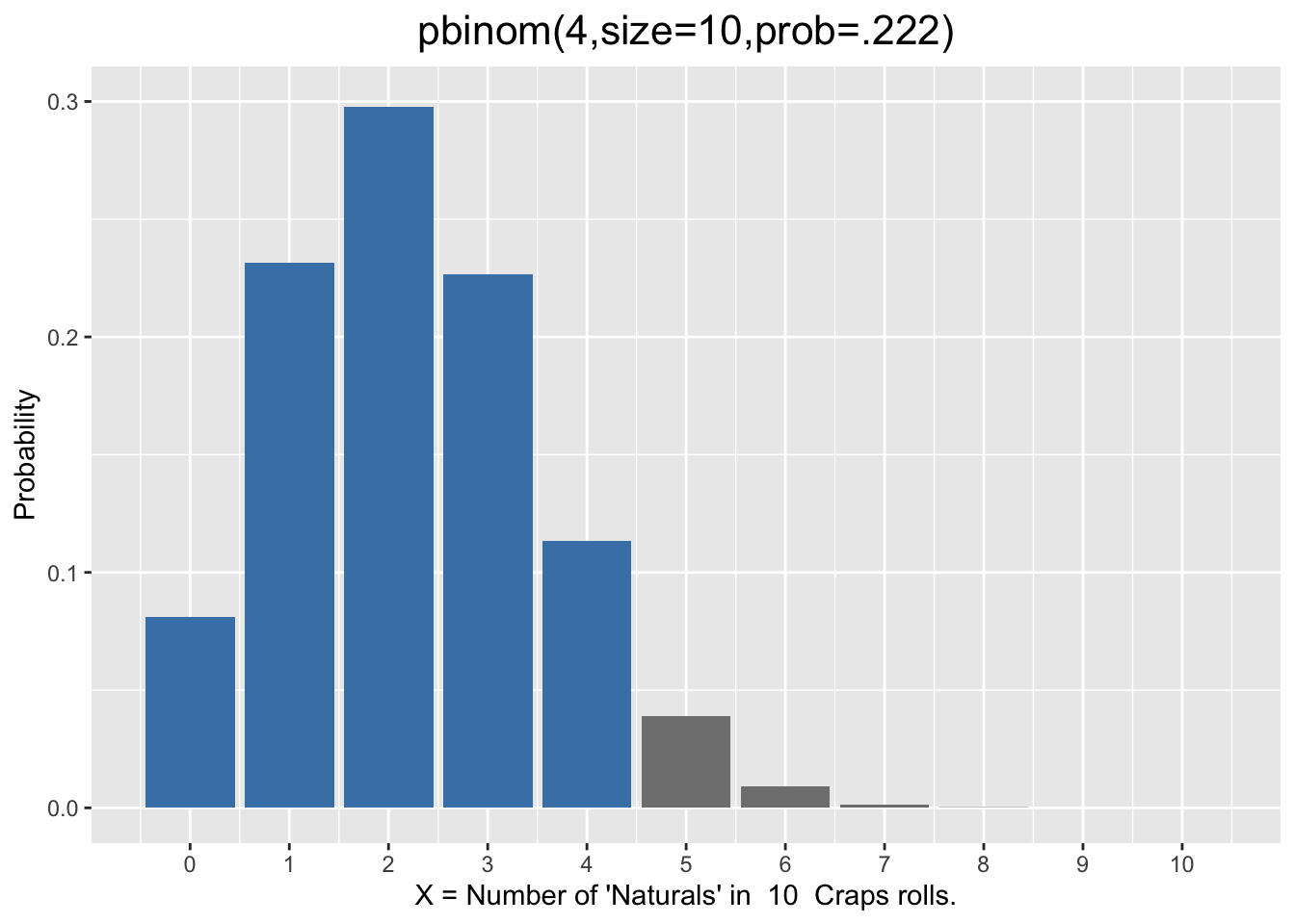
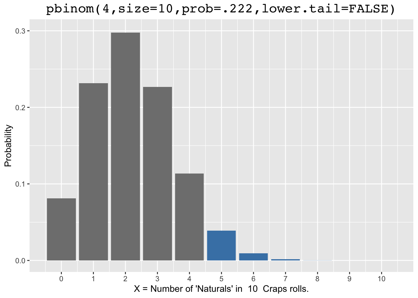
Figure 2.3: Left and Right Tail Probabilities

Notice on the right that adding lower.tail=FALSE to the pbinom() function call causes it to calculate the right tail probability \(P(X>4)\) (strictly greater). That seems strange since the left tail probability calculation was \(P(X\le4)\) (includes =). That is a subtlety that you have to be careful with if you calculate right tail probabilities for discrete distributions. The function works like that so that the total is 1 (sum of all bars). That is, you can calculate one from the other:

\[ pbinom(4, size=10, prob=.222 ,lower.tail=FALSE) \;\;\;=\;\;\; 1 - pbinom(4, size=10, prob=.222)\]

Understanding this, \(P(X\le4)\) can be calculated using either approach (left or right). It’s worth spending a bit of time to understand why both calculations below give the same result.

# P(X≤4) - P(X≤3)
pbinom(4, size=10, prob=.222) - pbinom(3, size=10, prob=.222) 
## [1] 0.113112
# P(X>3) - P(X>4)
pbinom(3, size=10, prob=.222, lower.tail=FALSE) - pbinom(4, size=10, prob=.222, lower.tail=FALSE)
## [1] 0.113112

Each of the discrete distribution examples we have presented have a finite number of possible outcomes. Some discrete distributions have an infinite number of possible outcomes, such as a Poisson distribution where each non-negative integer is a possible outcome. In such a case, there are an infinite number of bars in the distribution. Since all the bars must add up to 1 for ANY discrete distribution, the bar heights necessarily form an infinite sum which adds up to 1. However, such distributions are beyond the scope of this chapter.

2.4 Continuous Probability Distributions

Fundamentally, a continuous distribution is a continuous function that maps real numbers to real numbers: \(f: \mathbb{R}\rightarrow\mathbb{R}\) or perhaps \(f:[a,b]\rightarrow\mathbb{R}\). In the first case, the domain of the function is the whole real number line, and in the second case the domain is an interval of real numbers. Calculus books contain technical definitions for continuity, but the concept is simply that you can draw the “curve” without picking up your pencil. For such a function to qualify as a probability distribution, it must have a total area of 1 “under the curve.”

A continuous Uniform Distribution is the most simple continuous distribution, and thus a good choice to proceed by example. In general, a continuous uniform distribution is a constant function defined on an interval real numbers: \(f:[a,b]\rightarrow\mathbb{R}\). Constant function means \(f(x)=K\) for some number K for any x in the interval \([a,b]\).

Figure 2.4 shows a specific continuous uniform distribution \(f:[0,6]\rightarrow\mathbb{R}\). A uniform continuous distribution defined on \([0,6]\) must necessarily be the constant function where \(f(x)=1/6\), since the total area under the curve must be 1. That is, the shaded rectangle below has area \(6\times1/6=1\).

Figure 2.4: Continuous Uniform Probility Distribution on [0,6]

Probabilities are given by areas under the curve rather than adding up bars as with a discrete distribution. Since the curve is flat, such areas are rectangles. For example, \(P(X \le 2) = 2 \times 1/6 = 1/3\). That is, a there is a \(1/3\) probability that a random variable \(X\) selected from this distribution is in the interval \([0,2]\).

Having seen a concrete example, there is now sufficient context to list properties that hold for ALL continuous probability distributions.

Properties of Continuous Distributions:

• The total area under the curve is 1
• Probabilities of events are areas under the curve, where an event is a subset of the function’s domain.
• The probability of any single outcome is 0. That is, \(P(X=r)\) is \(0\) for any real number r.

The discussion surrounding Figure 2.4 has already demonstrated the first two properties above. We’ll also use that example to explain the third property, which might seem strange at first. For example, \(P(X = 3) = 0\). The key is that probabilities for continuous distributions are two-dimensional areas. There is no two-dimensional area above a single number. In Figure 2.4, the width of the base of such a rectangle is 0.

Another way to rationalize that is to suppose that each number on the x-axis in Figure 2.4 has a non-zero probability, perhaps \(1/6\). Then the probability of an event like the following would be infinite:  \(P(X=\frac{1}{2} \textrm{ or } X=\frac{1}{3} \textrm{ or } X=\frac{1}{4} \textrm{ or } \cdots)=1/6+1/6+1/6+ \cdots = \infty\) But that violates a fundamental rule of probability that \(0\le P(E)\le1\) for any event E. Looking at it another way, the event is a subset of the certain event \(0\le X\le 6\), which provides a contradiction since \(P(0\le X\le 6)=1\).

The concept of the mean (expectation) of a continuous distribution is basically the same as for a discrete distribution.

Mean of a Continuous Distribution:

Visually speaking, the mean can be thought of as an x-axis fulcrum point that balances the distribution’s total area under the curve as if it were a solid mass.

There are mathematical formulas for means (and standard deviations) of continuous distributions. But for the simple case of a uniform distribution, we can visually determine that the mean is exactly in the middle because of symmetry. For the distribution in Figure 2.4 the mean is 3, which would effectively balance the shaded rectangular block.

The punif() (probability uniform) function calculates the left tail probability for a continuous uniform distribution defined on the interval \([min,max]\). For example, the function calls below calculate the shaded areas shown in Figure 2.5.

# P(X≤2) 
punif(2, min=0, max=6)   # Uniform Distribution on [0,6]
## [1] 0.3333333
# P(X≤2 or X≥4) (three different calculations)
punif(2, min=0, max=6) + punif(4, min=0, max=6, lower.tail=FALSE)
## [1] 0.6666667
2* punif(2, min=0, max=6)  # Requires symmetry
## [1] 0.6666667
punif(2, min=0, max=6) + (1 -punif(4, min=0, max=6))  
## [1] 0.6666667

Figure 2.5: Probabilities for a Uniform Distribution on [0,6]

Of course, the probabilities in Figure 2.5 could easily be calculated simply as areas of rectangles rather than using punif(). But probabilities for non-uniform continuous distributions are not so readily calculated, so it’s important to get used to using left tail probability functions in R. In particular, it’s worth spending a minute to understand why the three different calculations above for \(P(X≤2\;or\;X≥4)\) all give the same result.

When dealing with probabilities, it’s also important to not forget the distinction between and/or. For example, for the uniform distribution above, \(P(X≤2\;and\;X≥4) = 0\) (because a single observation \(X\) can’t satisfy both conditions) and \(P(X≥2\;or\;X≤4) = 1\) (because \(X\) in \([0,6]\) satisfies both conditions).

This section concludes with a brief look in Figure 2.6 at some of the most commonly used continuous distributions in statistics.

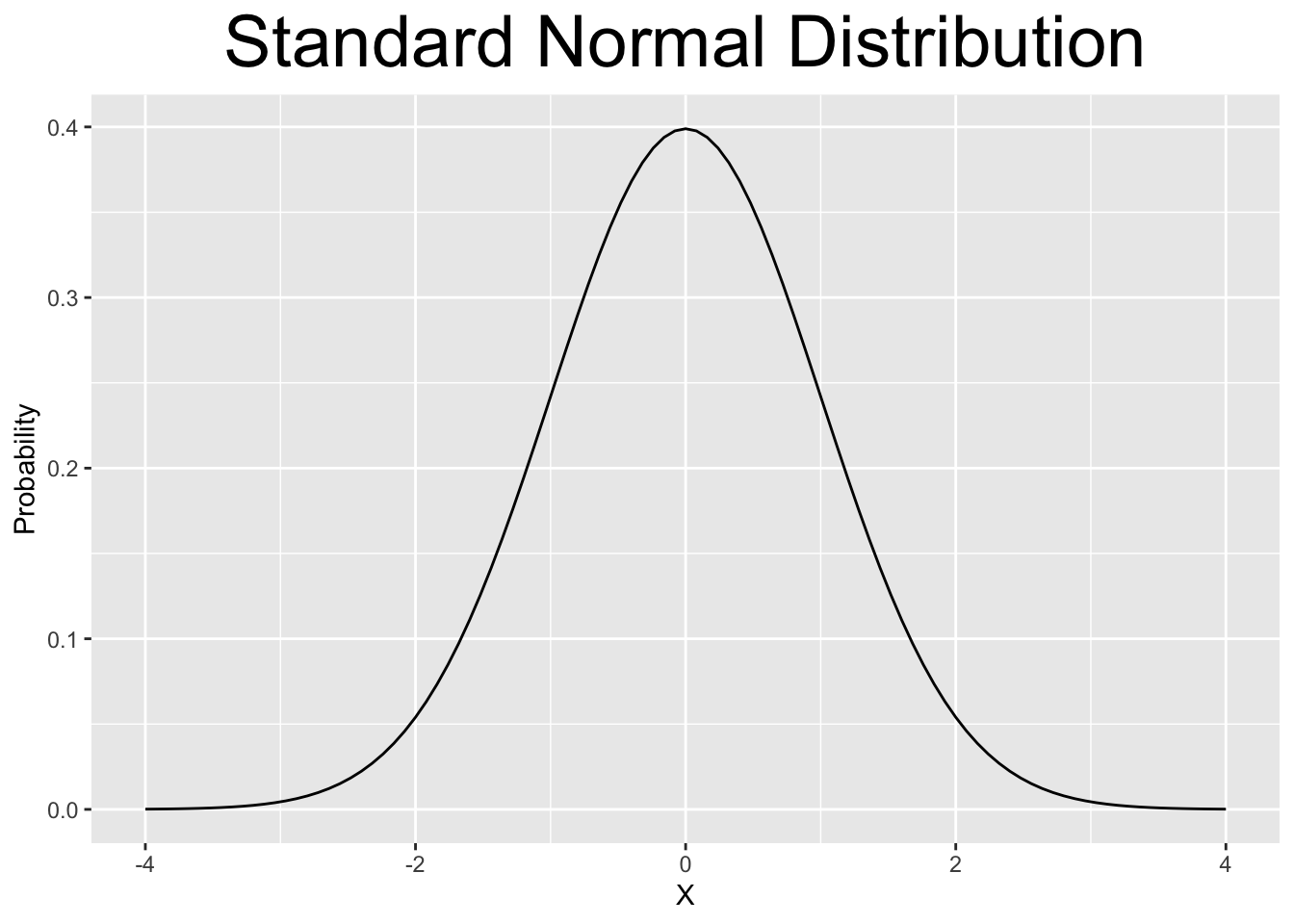
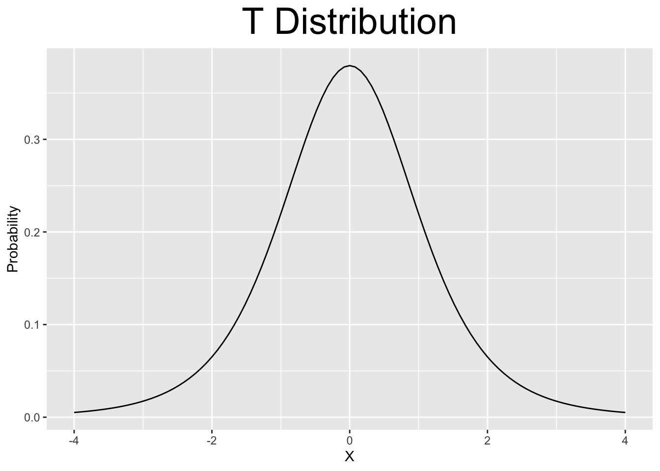
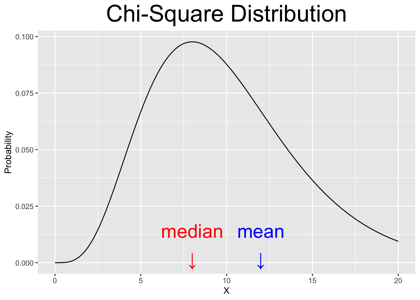
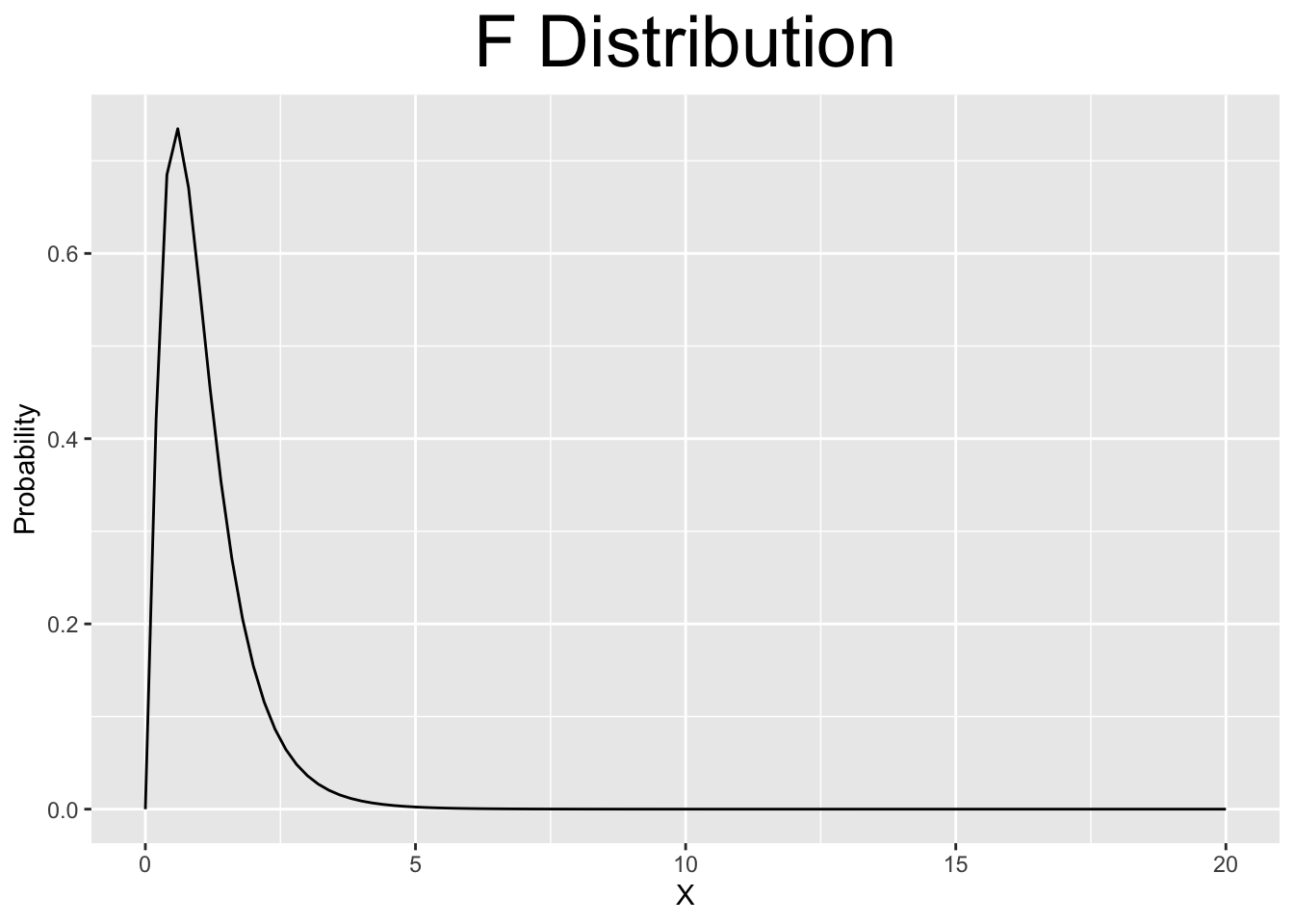
Figure 2.6: Various Continuous Distributions

More will be said about these distributions when they become relevant to the statistical analyses explored in the chapters to follow. But for now just some quick observations. First, all of them have total area 1 under the curve. Otherwise they would not be probability distributions!

The Standard Normal and T distributions are both symmetric and centered at 0 (mean \(\mu=0\)). They look almost identical, but the T distribution has slightly more area (probability) away from 0 out in the left and right tails. That can be seen (but barely) since both plots use the same x-axis scale. Both of them are defined on the entire real number line \((-\infty,\infty)\) and decrease asymptotically (gradually) towards \(\pm \infty\).

The \(\chi^2\) (pronounced Chi-Square) and F distributions are definitely not symmetric. Both of them are defined on the non-negative real numbers \([0,\infty)\) and decrease asymptotically (gradually) towards positive \(\infty\).

Left vs Right Skew:

The Chi-Square distribution in Figure 2.6 is skewed right since its mean is to the right of its median. That seems counter-intuitive since the hump (tallest part) is on the left. Skew direction is the opposite of the way the distribution appears visually.

2.5 Normal Distributions

Perhaps the most important continuous distribution is the normal distribution, also called a bell curve. You typically don’t need to work directly with the mathematical function for a normal distribution (unless you are in an advanced math course), but it’s worth seeing to emphasize that normal distributions are indeed a special type of mathematical function. A normal distribution is the function \(f:\mathbb{R}\rightarrow\mathbb{R}\) defined below whose domain is the entire real number line.

PDF for the Normal Distribution	Mean	Variance
\(f(x) = \frac{e^{-(x - \mu)^{2}/(2\sigma^{2}) }} {\sigma\sqrt{2\pi}}\)	\(\mu\)	\(\sigma^2\)

The acronym PDF stands for Probability Density Function, not to be confused with PDF Portable Document Format computer files (.pdf). Think of density in this context as the concentration of the area under the curve. For a uniform distribution (constant function), the probability density is distributed uniformly across the domain \([a,b]\) of the function. For a bell curve, most of the probability density is concentrated in the bell-shaped region in the center.

The standard notation for a normal distribution is \(N(\mu,\sigma^2)\). The Greek letter \(\mu\) represents the mean of the distribution and \(\sigma\) represents the standard deviation, which for simplicity is often abbreviated as sd. The quantity \(\sigma^2\) is called the variance of the distribution.

Figure 2.7 shows four normal distributions to demonstrate these concepts. They could also be listed as \(N(0,1^2)\), \(N(0,.5^2)\), \(N(0,2^2)\), and \(N(5,1^2)\). It is often convenient to use the “squared notation” to make the standard deviation readily apparent. Obviously, the variance and sd can be calculated from each other, so why are two different quantities used that both measure the spread (how wide or narrow) of the distribution? Depending upon the particular computation, each of \(\sigma\) and \(\sigma^2\) are very useful in formulas and theorems in the mathematics of probability theory. However, \(\sigma\) is generally more intutitve to humans when considering the spread of a distribution.

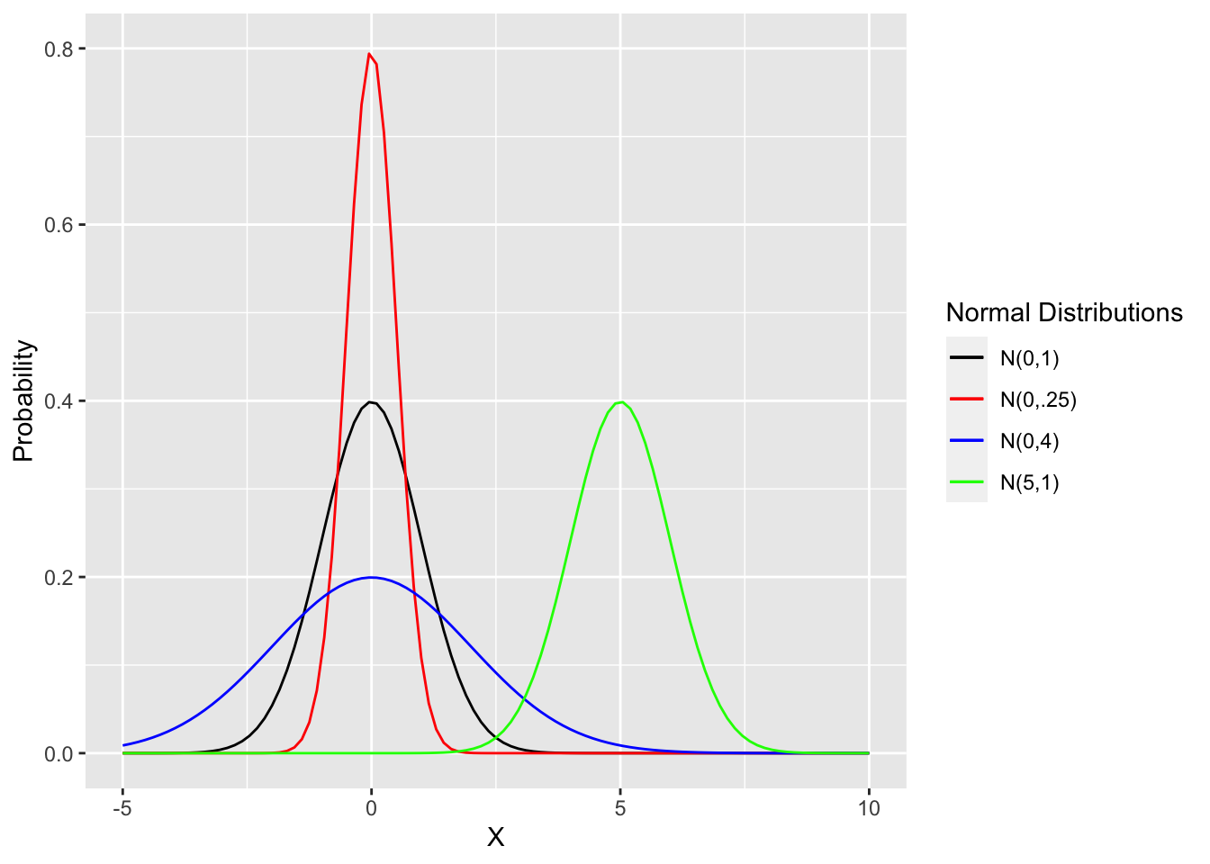
Figure 2.7: Comparison of Different Normal Distributions

The black one with \(\mu=0\) and \(\sigma=1\) is called the Standard Normal Distribution. Observe that the red and blue distributions also both have \(\mu=0\), but have different variances. The smaller the variance, the more narrowly the distribution is concentrated around the mean. That is, the smaller the variance, the more probability is concentrated in the middle near the mean \(\mu\) with less probability in the “tails” that asymptotically (gradually) decrease towards \(\pm \infty\).

The green distribution has the same variance as the standard normal distribution, hence the same shape, but has a different “center” at \(\mu=5\). Note that it only makes sense to say the mean is the “center” of a distribution if the distribution is symmetric, meaning the distribution is a mirror image around the mean.

It can be proven mathematically that if a random variable \(X\) is normally distributed \(N(\mu,\sigma^2)\), then the random variable \(Z\) as defined below is Standard Normal. That implication is shown below.

\[ \text{Distribution of } \; X \; \text{ is } \; N(\mu,\sigma^2) \;\;\;\;\;\;\implies\;\;\;\;\;\; \text{Distribution of } \; Z=\frac{X-\mu}{\sigma} \; \text{ is } \; N(0,1) \]

The random variable \(Z\) as defined above is called the normalization of \(X\) and the Standard Normal \(N(0,1)\) is often called the Z Distribution.

For a specific example, suppose \(X\) is distributed \(N(3,2^2)\). The value of \(X=6\) can be normalized by computing its z-score as shown below.

\[Z=\frac{6-3}{2} = 1.5\]

On the surface, it’s not intuitive how the value of \(X=6\) relates to a \(N(3,2^2)\) distribution. But a closer look reveals that \(6=3+1.5\times 2=\mu+1.5\times\sigma\), meaning that \(X=6\) is exactly 1.5 standard deviations greater than the mean \(3\). Thus, the z-score effectively measured how many standard deviations above the mean a value of \(X=6\) is. Again, saying \(X=6\) comes from a \(N(3,2^2)\) distribution is just throwing out some numbers, but saying \(X=6\) has a x-score of 1.5 in a \(N(3,2^2)\) distribution says something far more intuitive.

Figure 2.8 shows probabilities (blue shaded areas) related to the discussion just above. The plot shows the left tail probability for \(P(X\le 6)\) on the left and the corresponding normalized probability \(P(Z\le 1.5)\) on the right.

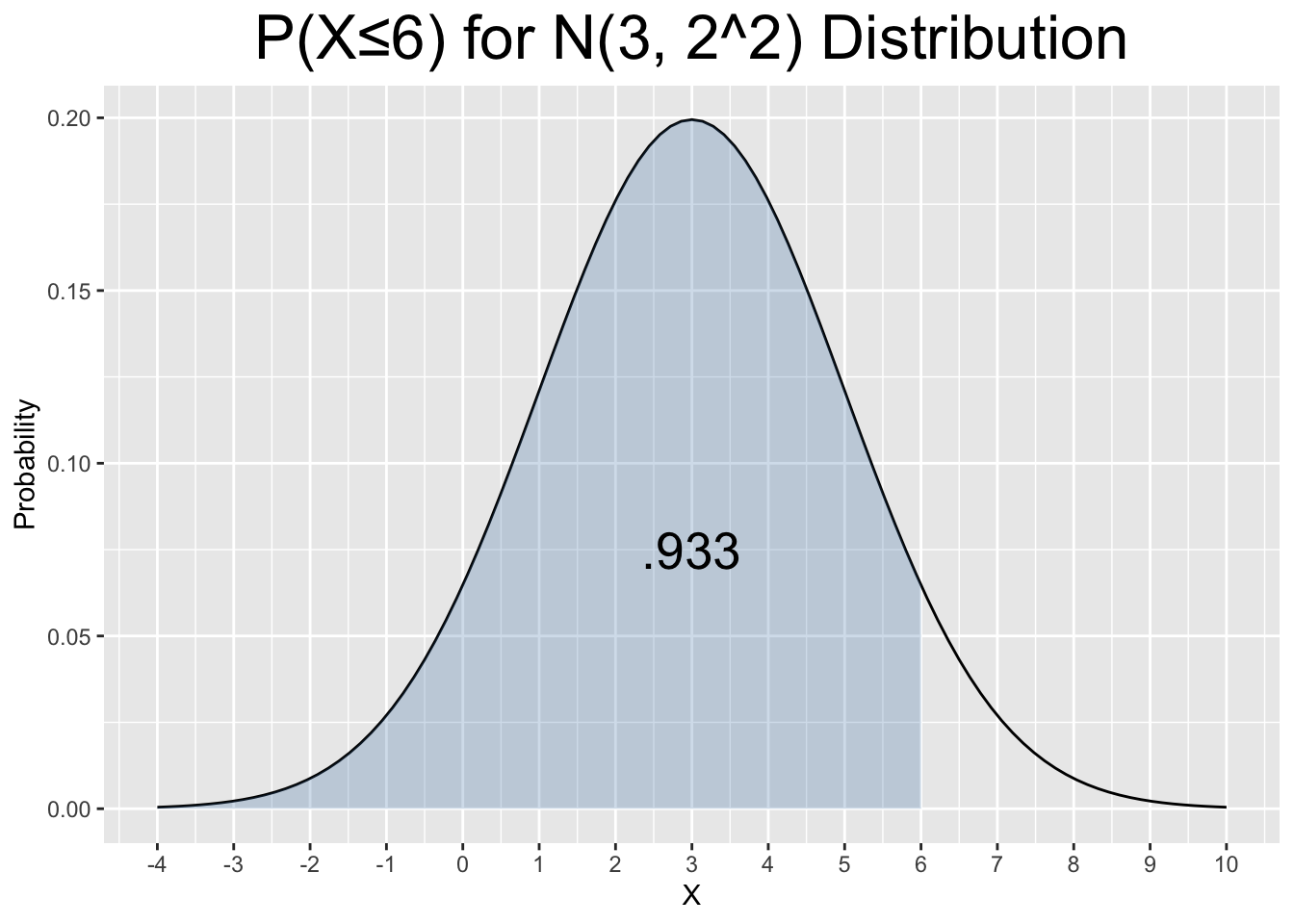
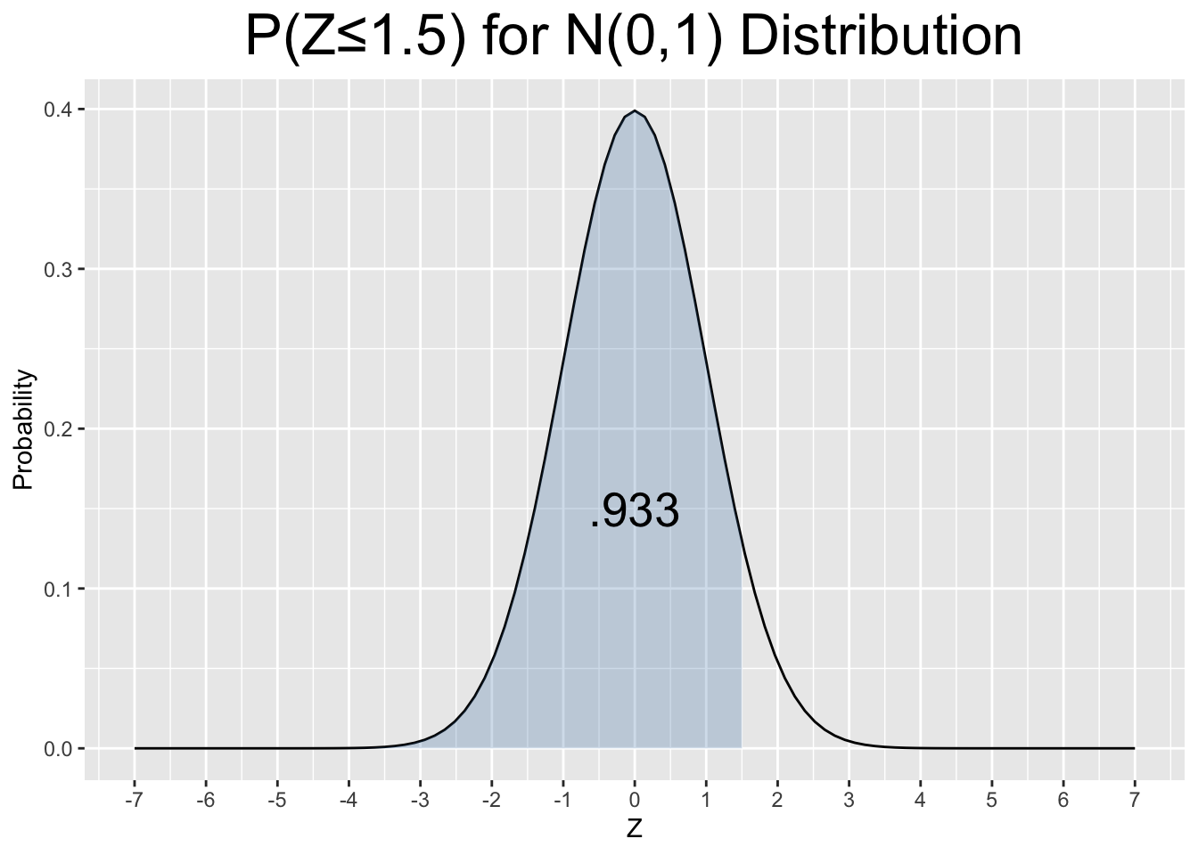
Figure 2.8: Using a Z-Score to Normalize a Probability Calculation

If you have read the previous sections in this chapter, it should not surprise you that that R provides a pnorm() (probability normal) function that computes left tail areas for normal distributions. Both blue-shaded probabilities shown in Figure 2.8 are computed below.

pnorm(6, mean=3, sd=2)    # P(X ≤ 6) for N(3,2^2)
## [1] 0.9331928
pnorm(1.5, mean=0, sd=1)  # P(Z ≤ 1.5) for N(0,1) Standard Normal
## [1] 0.9331928

It is no coincidence that the two probabilities are equal: \(P(X ≤ 6) = P(Z ≤ 1.5)\). Simply put, \(P(X ≤ 6)\) was equivalently calculated using the normalization. We now state that concept more formally.

Suppose the random variable \(X\) is distributed \(N(\mu,\sigma^2)\). Then the following follows from z-score normalization.

\[P(X\le x_0)=P(Z\le z_0) \;\;\;\;\;\; \text{ where } \; z_0=\frac{x_0-\mu}{\sigma}\] This says that the \(N(\mu,\sigma^2)\) probability that \(X\le x_0\) for some value \(x_0\) is equal to the corresponding \(N(0,1)\) normalized probability where \(z_0\) is the z-score for \(x_0\). The principle above features a left tail probability, but the same principle applies to more complex probabilities. That means that ANY probably calculation for a \(N(\mu,\sigma^2)\) distribution can be normalized and calculated using the Standard Normal distribution \(N(0,1)\).

Historical Note:

In the pre-computing era, statistics books would contain a probability lookup table for the standard normal Z Distribution. In order to compute \(P(X ≤ 6)\) for a \(N(3,2^2)\), you would have to normalize the problem and then look up the probability in the Z table. Therefore, one needed to constantly compute z-scores. But now with computing convenience at your fingertips, it actually takes more work to normalize the problem than to directly compute a non-\(N(0,1)\) probability.

Before moving on, its worth re-emphasizing some continuous distribution probability nuances in the context of normal distributions. Probabilities for individual outcomes such as \(P(X=6)\) are always 0 since there is no two-dimensional area under the curve. Thus, \(P(X\le 6)=P(X< 6)\), for example, although it usually seems more natural to write it the first way. Since normal distributions are symmetric (mirror image about the mean), a right-tail probability such as \(P(X\ge -6)\) can be computed by \(P(X\ge -6)=P(X\le 6)\) where the right side is easier to compute using pnorm() since it involves a left tail area. Or using the fact that the total area under the curve is 1, \(P(X\ge -6) = 1-P(X\le -6)\) again switching to a left tail calculation on the right.

The 68-95-99.7 Rule stated below gives insight into how the probability density under a normal curve relates to the standard deviation. Figure 2.9 provides a graphical depiction of the rule.

68-95-99.7 Rule for Normal Distributions

For ANY normal distribution, approximately 68%, 95%, and 99.7% of the X values lie within 1, 2, and 3 standard deviations of the mean, respectively. It is sometimes called the 68-95-99 Rule for simplicity and it ONLY applies to normal distributions.

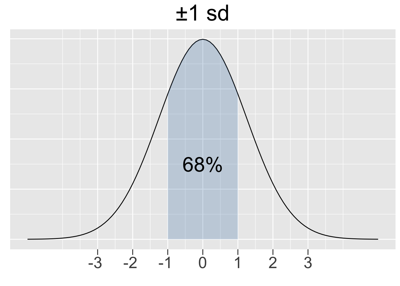
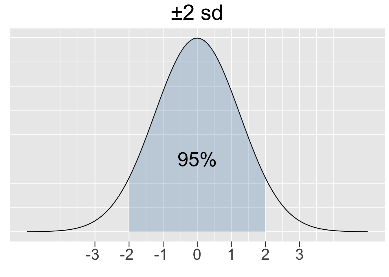
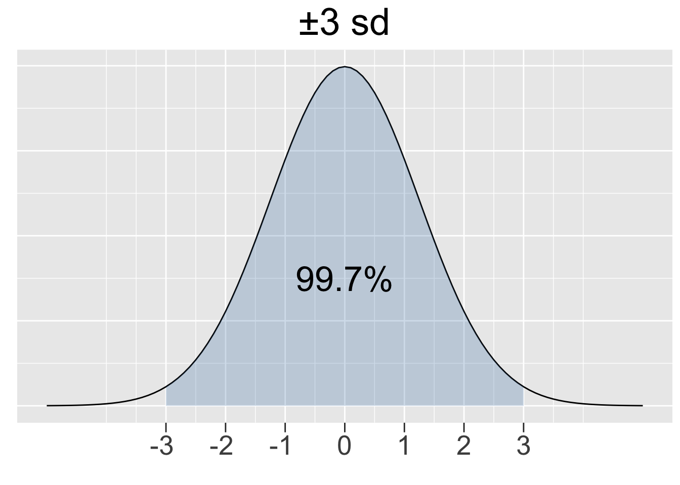
Figure 2.9: Illustration of the 68-95-99.7 Rule for Normal Distributions

The R code below calculates the shaded areas shown in Figure 2.9. Drawing upon the mathematics behind normalization, it is sufficient to do the calculations for the standard normal \(N(0,1)\).

# Calculations for a N(0,1) standard normal distribution
1-2*pnorm(-1, mean=0, sd=1)  # ±1 sd on each side of mean
## [1] 0.6826895
1-2*pnorm(-2, mean=0, sd=1)  # ±2 sd on each side of mean
## [1] 0.9544997
1-2*pnorm(-3, mean=0, sd=1)  # ±3 sd on each side of mean
## [1] 0.9973002

The pnorm() calculations above might look a bit strange, but each uses only one call to pnorm(). For example pnorm(-1) is a left tail area, so by symmetry 2*pnorm(-1) adds the corresponding right tail area. The area in the middle shown in Figure 2.9 is then 1- 2*pnorm(-1).

The more natural way (although less efficient) to compute a “between the tails area” is shown below. This time the computations are for an arbitrarily chosen \(N(-10,5^2)\) distribution and gives the same result (just in case you were skeptical about the 68-95-99 Rule).

# Calculations for a N(-10,5^2) normal distribution
pnorm(15, mean=10, sd=5) - pnorm(5, mean=10, sd=5)  # ±1 sd on each side of mean
## [1] 0.6826895
pnorm(20, mean=10, sd=5) - pnorm(0, mean=10, sd=5)  # ±2 sd on each side of mean
## [1] 0.9544997
pnorm(25, mean=10, sd=5) - pnorm(-5, mean=10, sd=5) # ±3 sd on each side of mean  
## [1] 0.9973002

2.6 P-Q-R-D Distribution Functions

The strange title of this section refers to the “family” of functions specific to each probability distribution. For example consider the p-q-r-d functions for the normal distribution: pnorm() (probability), qnorm() (quantile), and rnorm() (random), and dnorm() (density).

We’ll simply refer to this collection of functions as the *-norm family, or perhaps p-q-r-d-norm. Figure 2.10 provides an illustration to help demonstrate how the *-norm family of functions work.

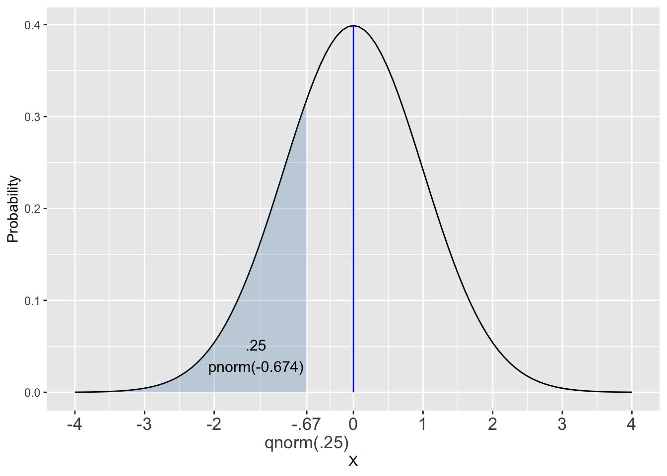
Figure 2.10: Illustrating the p-q-r-d-norm Family of Functions

The code below shows a call to each of the *-norm functions. Each function call uses the parameters of a standard normal distribution \(N(0,1)\) to match the diagram.

# Area of blue-shaded left tail
pnorm(q = -0.6744897502, mean = 0, sd = 1)   # Probability
## [1] 0.25
# X-axis value defining blue-shaded left tail
qnorm(p = .25, mean = 0, sd = 1)             # Quantile
## [1] -0.6744897502
# 3 random numbers from N(0,1) Distribution
rnorm(n = 3, mean = 0, sd = 1)               # Random
## [1] -0.8204683841  0.4874290524  0.7383247051
# Height of vertical blue Line = f(0) value from Probability Density Function
dnorm(x = 0, mean = 0, sd = 1)               # Density
## [1] 0.3989422804

You should be well aware of how pnorm() works, having seen several “p-functions” in previous sections. Observe in Figure 2.10 that qnorm() is the inverse function (mathematically speaking) of pnorm(). Plug an x-axis value into pnorm() and it spits out a probability area. Plug that area back into qnorm() and it spits back the same x-axis value.

In this context the x-axis value, is considered a quantile for the distribution. In this example, \(q=-0.67\) is the 25th percentile for a \(N(0,1)\) distribution. In Figure 2.10, the function calls are denoted as pnorm(q) and qnorm(p) to emphasize the p’s and q’s so to speak. Previously in this chapter we had been omitting the name of the first value passed to the function, as in pnorm(-0.67) (which is the same as pnorm(-0.67, mean=0, sd=1) since pnorm() defaults to \(N(0,1)\) if not told otherwise.)

Median of a Probability Distribution

The 50th percentile (half of the area on each side) of a probability distribution is its median. The median and mean are equal if and only if the distribution is symmetric. For example, if the distribution is skewed left (hump on right) the median is more toward the right (hump has more than 50% of the area) leaving the mean to the left of the median.

Subsequent chapters will highlight the rnorm() function, and random number generating “r functions” for other distributions as well. For now, we’ll provide a quick example to re-emphasize the z-score concept.

The code below generates 1 random value from a \(N(-7.37,(.88)^2)\) normal distribution and then calculates the corresponding z-score. The normal distribution has non-intuitive mean and sd to demonstrate that the z-score is the more intuitive quantity than the random value itself.

x <- rnorm(1, mean=-7.37, sd=0.88)   # 1 random number from N(-7.37,(.88)^2)
z <- (x - -7.37)/0.88                # z-score for x
cat("Random Observation x:", x, "  Calculated z-score:", z)
## Random Observation x: -5.36   Calculated z-score: 2.29

The quick observation is that the random value -5.36 is more than 1 standard deviation (.88) away from the distribution mean -7.37. Aside from that, the numbers in the previous sentence don’t carry intuitive meaning for a human. However, the z-score is much more telling: the random outcome is just over 2 sd’s greater than the mean. Recalling the 68-95-99.7 rule, the random value is just outside of the middle 95% of the area under the curve (among the 5% of “unusual” values) but not outside the the middle 99.7% area (but not among the .3% of “extreme” values).

The moral of this example is that z-scores provide intuitive perspectives about a value from normal distributions in terms of how ordinary or unusual or extreme the value is relative to the expectation. Should one need more precision, a quick calculation using qnorm() shows the random value -5.36 is at about the 99th percentile of the \(N(-7.37,(.88)^2)\) distribution.

Try it!

Copy all 3 lines of the above code and paste them into your RStudio Console (or R script). Run all 3 lines of code several times (don’t forget the ↑ console shortcut) and observe the z-scores. Acording to the the 68-95-99.7 rule, you should get a z-score in the \(z<-2 \; or \; z>2\) range about 5 out of 100 tries (1 out of 20) and outide the \(\pm3\) range only about 3 out of 1000 tries. How lucky are you feeling today?

This section concludes by summarizing the p-q-r-d “Family” of functions for the distributions you will encounter in subsequent chapters. Core R (no package needed) does provide p-q-r-d functions for other, less common distributions as well. For each distribution below, the q-*, r-*, and d-* versions use the same format as p-* functions that are listed.

Distribution	Required Arguments (using p)
Binomial Uniform Normal T \(\chi^2\) F	pbinom(q,size, prob) punif(q,min,max) pnorm(q,mean,sd) pt(q,df) pchisq(q,df) pf(q,df1,df2)

Note that the examples on the right show the required arguments necessary to tell the function the exact shape of the distribution. You might be curious what the “df” (degrees of freedom) arguments are above. That quantity defines the shape of some distributions functions, and will be discussed in subsequent chapters.

2.7 Distribution Plots

You may have noticed that the previous section basically skipped over discussion of the “density functions” such as dnorm() other than finding the apex (maximum) of the Standard Normal distribution with dnorm(0). That was certainly easier than finding it using calculus on the Standard Normal PDF function that was shown at the beginning of Section 2.5. Although that would be good fun on a rainy day.

The mathematical theorems in statistics theory relies heavily on such PDFs, but doing statistical analyses rarely, if ever, require directly using them. So there’s no compelling reason to discuss them in detail here. However, since these chapters focus on computational statistics, perhaps showing how dnorm() was used to draw the normal curves in this chapter will alleviate some of your curiosity.

The code and resulting plot below use the ggplot2 stat_function() to draw a \(N(0,1)\) curve in one plot layer and adding shading with another layer. Both times stat_function() is passed the dnorm density function name to tell it what function to plot.

# Define the x-axis limits for the Plot
# ggplot needs a data table as argument
 x_axis <- tibble(
  xlim = c(-4, 4)
)
ggplot(x_axis , aes(x = xlim)) +
   stat_function(fun = dnorm, args = list(mean = 0, sd = 1)) +
   stat_function(fun = dnorm, args = list(mean = 0, sd = 1), 
        geom = "area", fill = "steelblue", alpha = .25, xlim=c(-4,0))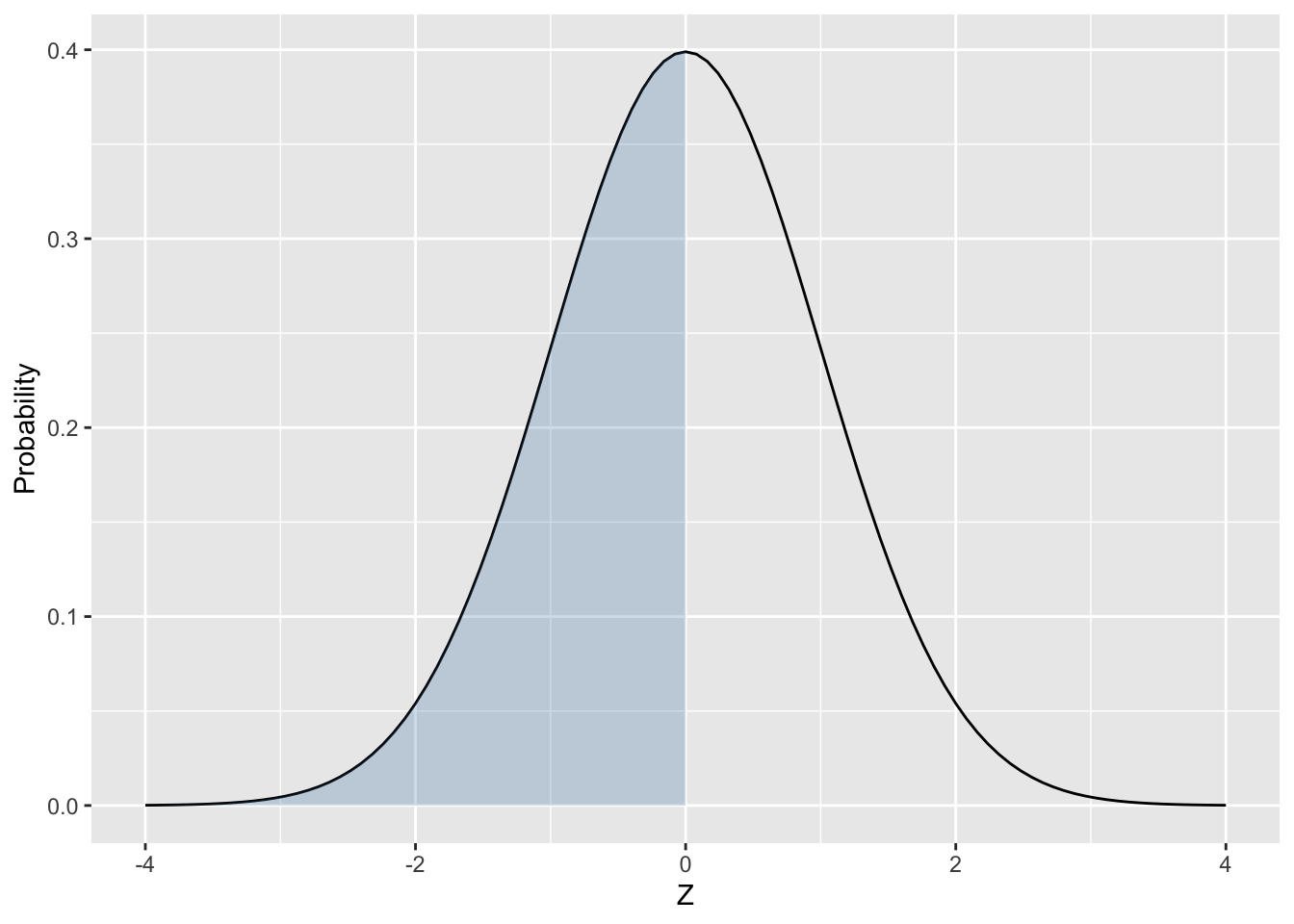

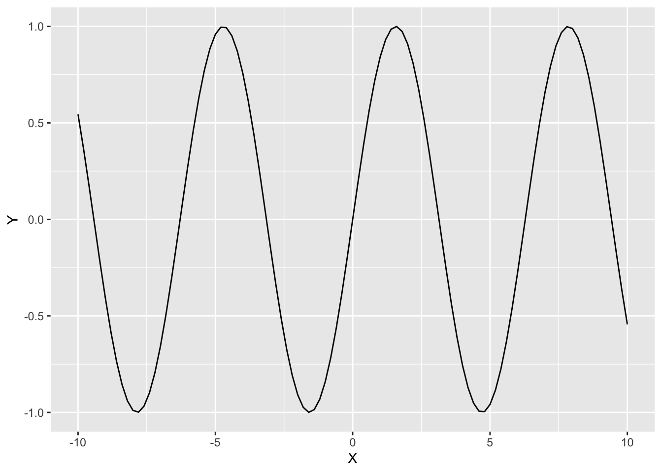
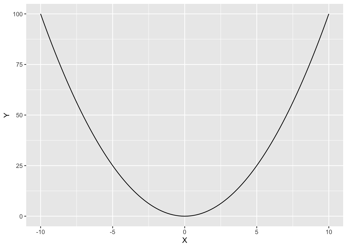
As a final note, stat_function() can be used to plot many types of functions, not justd-* probability density functions. For example, R recognizes many common mathematical functions, such as trigonometric functions like sin(), cos(), and tan(), as well as functions you define yourself. The code below plots a trig function and also a self-defined function that squares numbers. If you were to call the self-defined x_squared(3) the result is 9. But rather than calling it, the code below plots it.

# Define the x-axis limits for the Plot
# ggplot needs a data table as argument
x_axis <- tibble(
  xlim = c(-10, 10)
)

# Plot of sin() (core R)
ggplot(x_axis , aes(x = xlim)) +
   stat_function(fun = sin)

# Self-defined function named x_squared
x_squared <- function(x) {x*x}

# Plot of x_squared() (self-defined)
ggplot(x_axis , aes(x = xlim)) +
   stat_function(fun = x_squared)